Lab 19: Catchment Analysis
Chani Welch and Fes de Scally
Catchments, also known as watersheds and drainage basins, are fundamental units of the terrestrial landscape. Their boundaries are system boundaries for hydrological, geomorphological, and ecological processes. In brief, all precipitation that falls on a catchment drains to a single low, outlet point. This movement of water creates physical connections between all parts of a catchment. As a result, activities in one part of a catchment can influence water movement in another.
In this lab you will explore catchment attributes that control the rate and timing of surface water flow through catchments. You will differentiate hydrographs produced in response to rainfall based on catchment attributes. You will gather your own measurements of catchment characteristics using Toporama and analyze the data at two different scales.
Learning Objectives
After completion of this lab you will be able to:
- Understand and predict some of the effects of catchment attributes on stream discharge.
- Understand links between surface water and groundwater in catchments.
- Delineate a catchment using online mapping platforms.
- Measure and analyze catchment and stream network attributes using online mapping tools.
- Understand and predict the effects of map scale on the perceived complexity of the catchment and stream network and measured attributes.
Pre-Readings
Catchments as Systems
At the global scale, the hydrological cycle describes the movement of water between continents, oceans, and the atmosphere. Hydrologists and geomorphologists are generally more interested in assessing the hydrological cycle at the smaller scale of catchments. Catchments are a unique areal unit of the terrestrial landscape. The various names we use for this physical unit provide clues as to why catchments are unique units:
- Catchment: This area catches all water that falls onto it as precipitation.
- Watershed: This area sheds all water that falls on it to a single point.
- Drainage basin: All water that falls onto this area drains to a single point.
In summary, a catchment may be defined as an area of land that drains all water to a single outlet point. The outlet is the lowest point in the catchment. In other words, water moves from areas of higher elevation to areas of lower elevation. The boundary of a catchment is called a drainage divide, as it divides drainage into one catchment or another. It can be visualized as the highest point of land separating one catchment from adjacent catchments. Sediment eroded from a catchment by glacier ice or running water cannot be transported across the drainage divide into an adjacent catchment by water movement. Likewise, fish cannot migrate over a divide into an adjacent catchment.
Most commonly, the outlet of a catchment is a river mouth, where the river discharges water and sediment into the downstream lake, river, or ultimately, the ocean. In contrast, the outlet of some catchments is a depression in the landscape that forms a lake (at least some of the time). This type of catchment is called a closed catchment. All precipitation that falls on this type of catchment flows to the outlet where it either evaporates or infiltrates into the ground. A local example of this type of catchment is White Lake, south-east of Penticton, BC.
Drainage Networks
Each catchment contains a stream network that channels surface water to the catchment outlet. Depending on the size of the catchment, these streams range in number from one or two to tens of thousands. Each catchment has a main stream into which tributaries deposit water and sediment. The smallest tributaries, furthest from the catchment outlet, are called headwater streams. These are the streams where rivers begin. Although they carry smaller volumes of water, they often cover a significant portion of the total length of streams in a catchment, and play important roles in recharging groundwater, containing flood water, improving water quality, and providing fish and wildlife habitat.
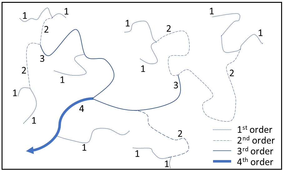
One way of assessing the complexity of a stream network is by ordering the streams in a catchment into a hierarchy. The most common method used to define stream order is the Strahler method (Figure 19.1):
- Starting at the uppermost points in the catchment, all headwater, or unbranched tributary streams are given a stream order of 1, and called first-order streams.
- When two first-order streams join, the stream order increases to 2 (second-order).
- When two second-order streams join, the stream order increases to 3, and so on.
Note that the stream order does not increase if two streams of different orders join. The highest stream order becomes the catchment order, so for example, Figure 19.1 depicts a fourth-order catchment.
The stream or drainage network can also be described on the basis of its shape, or drainage pattern. Different patterns are usually the result of structural or lithologic controls and include:
- Dendritic: develops in regions where there are no clear-cut structural or lithologic controls, i.e., areas with homogeneous geology. The most common drainage pattern and the most energy efficient because the length of tributaries is minimized.
- Trellis: develops in areas of strong structural or lithologic control, in particular where there are differentially eroded rock bodies and the streams flow along the strike of the less competent rocks that have been eroded. Tributaries flow down slopes to enter the main streams at right angles.
- Parallel: often develops on steep slopes. Tributaries are parallel to each other.
- Rectangular: develops in a faulted and jointed landscape, which directs stream courses in patterns of right angle turns.
- Deranged: develops where the original stream network has been disturbed, has no clear geometry, and no true stream valley. Particularly common on the Canadian Shield which was deeply scoured by ice sheets during the last glaciation.
Stream Discharge
The quantity of water flowing down a stream is called stream discharge. It is measured as a volumetric flow rate, most commonly cubic metres per second (m3/s, also known as cumecs). Discharge is commonly plotted against time; this is known as a hydrograph. Discharge is controlled by catchment size, shape and relief, drainage pattern and density, climate, land cover, in-stream controls, and the underlying geology.
Generally, as catchment size increases, discharge also increases. Major exceptions to this are 1) exotic streams that have their headwaters in temperate climates and lower reaches in arid climates, and 2) rivers that from which large quantities of water are removed by human activities. These two situations commonly occur in the same river system, such as the Columbia River system in North America.
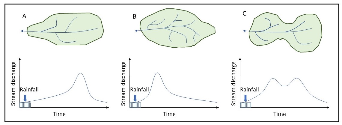
Catchments can possess an infinite variety of shapes, reflecting the history, structure and rocks of a region. Shape plays a major role in controlling the time sequence by which water enters the main stream of a catchment, and hence the timing of flood peaks (highest point on discharge curves; Figure 19.2). Elongated catchments tend to produce smaller flood peaks than rounded or tear-shaped catchments because the arrival of rainfall runoff at the mouth is staggered over a longer period of time (Figure 19.2c). In rounded or tear-shaped catchments (Figure 19.2a, b), runoff arrives at the mouth at more or less the same time from all tributaries.
Catchment relief, the difference in elevation between the highest and lowest parts of the catchment, is also controlled to a large degree by geological structure. A catchment with greater relief will have a faster runoff and discharge response to a rainfall event.
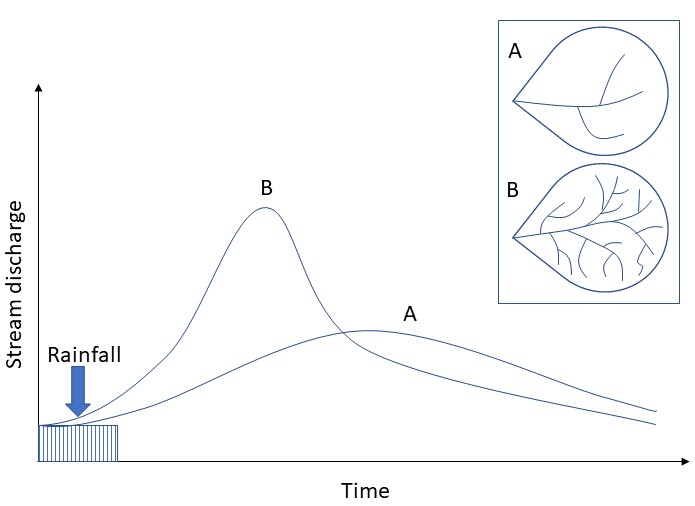
Drainage density is defined as the length of stream channels per unit area of a catchment. Drainage density reflects land use, underlying geology, and affects infiltration and the response time between rainfall and runoff. In general, higher drainage densities (Figure 19.3b) result in larger flood events because water travels shorter distances overland (a relatively slow process) before reaching a stream and hence less time to infiltrate into the ground when compared to catchments with lower drainage densities (Figure 19.3a). Because water reaches stream channels more quickly, higher drainage densities also lead to earlier flood peaks. In terms of geomorphology, it plays a role in the development of slopes.
Streams may be either perennial (always have discharge), intermittent (only discharge when there is enough water coming from upstream or groundwater, for example, glacier melt, usually seasonal) or ephemeral (only flow in response to rainfall events). The latter two are most common in arid environments. In-stream controls such as dams separate discharge at catchment outlets from rainfall events by controlling discharge to optimize power generation or minimize flood risk in downstream areas.
Land cover can affect drainage patterns (consider irrigation ditches, for example, or channelized portions of rivers) and the conversion of rainfall to infiltration versus runoff. Urban catchments, for example, tend to be covered with less permeable cover (concrete, rather than trees or grass), and so generate flood peaks that are higher and occur more quickly than an equivalent natural catchment.
Morphometric Attributes of Catchments
Catchment morphometrics (morpho = form; metrics = measures of) provide quantitative tools for comparing the control that catchment attributes have on the timing and rate of stream discharge. We will look at two catchment and one stream network metric.
One of the most common ways to measure catchment shape is using Schumm’s Elongation Ratio (E) (Equation 19.1):
[latex]E = \dfrac{D}{L}[/latex]
where D is the diameter of a circle with the same area as the catchment, and L is the horizontal distance along the longest axis of the catchment parallel to the main stream (Schumm, 1956).
Schumm (Schumm, 1956) also developed a simple measurement of catchment relief, known as Schumm’s Relief Ratio (R) (Equation 19.2):
[latex]R = \dfrac{H}{L}[/latex]
where H is the difference between the highest and lowest elevations in the catchment, and L is as defined above for E in Equation 19.1.
Note that E and R are both unitless. Ensure that D and L, or H and L have the same units prior to calculating. Common units are metres (m) or kilometres (km).
Drainage density (Dd) is defined as the length of stream channels per unit area of a catchment (units of km / km2 or km-1) (Equation 19.3):
[latex]D_{d} = \dfrac{L (km)}{A (km^{2})}[/latex]
where L is the total length of all streams in the catchment (in kilometres) and A is the area of the catchment (in square kilometres, km2).
Groundwater Connections
When precipitation falls on a catchment, some portion of the water may infiltrate into the ground, and continue below the root zone into groundwater. The amount of precipitation that reaches the groundwater is determined by the characteristics of the local geology, plant use, and the timing, volume and intensity of precipitation events.
Areas where precipitation infiltrates into groundwater are known as recharge areas, and areas where groundwater returns to the surface, for example, into a river or a lake as a spring, are known as discharge areas. Recharge and discharge areas are sometimes very close to each other (tens of metres) and sometimes hundreds of kilometres apart. They are sometimes contained within a single surface water catchment, and sometimes are not.
The types of geology that increase the amount of groundwater flow are those that contain very permeable rocks, or lots of fissures and fractures for water to easily flow through. Limestone is one example of a very permeable type of rock. Water flows more slowly through the subsurface than in surface streams due to the extra resistance provided by the rock or soil.
In many areas, surface water flow plays a more active role in landscape formation than groundwater, and hence is the focus of this lab. However, groundwater, or its removal, does also play an active role in shaping landscapes. For example, subsidence can occur when large amounts of groundwater are removed from an aquifer; the overlying land sinks, changing catchment relief. Groundwater springs also sustain headwater lakes and streams.
Introduction to Toporama
Toporama is an online mapping tool provided by Natural Resources Canada. The maps include:
- Ground relief.
- Lakes and rivers.
- Administrative and populated areas.
- Roads and transport facilities.
You can select the layers that you wish to display. You can also choose the base layer of your map (e.g., Canada Base Map or satellite imagery). Toporama enables you to measure features, annotate, and export maps of your own creation.
Please note that while Toporama is a wonderful tool, it can be slow to load. Your patience is appreciated. If you have persistent problems, clear your cookies/cache and/or reboot your computer.
Lab Exercises
In this lab you will analyze a catchment using tools available in Toporama. You will
- Learn how to delineate a catchment and assess this delineation.
- Measure catchment and stream characteristics at two different scales.
- Calculate catchment morphometrics.
- Assess the effects of catchment attributes on discharge.
You will need access to a computer with internet connection to access Toporama and a calculator. It is estimated that this lab will take 2-3 hours to complete, depending on your familiarity with Toporama.
EX1: Catchment Characteristics and Discharge
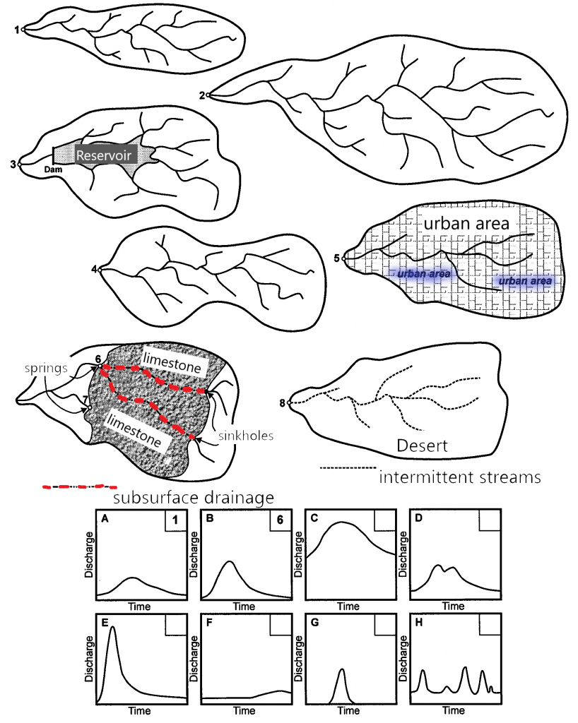
A number of lowland catchments (i.e. catchments with no appreciable relief) with different shapes, sizes and characteristics are shown on Figure 19.4. Assume that all catchments receive a similar amount of rainfall over a similar period of time from a summer storm. The hydrographs A to H in the lower half of the figure represent the discharge response of each catchment at the numbered locations.
- Match each catchment with the appropriate hydrograph, basing your choice on the catchment characteristics that affect the discharge: size, shape, stream network, surface land cover, underlying geology, and climate. Refer back to the introductory material as necessary.
EX2: Analyzing a Catchment at a Small Scale
Delineating a catchment is the first step in analyzing hydrological processes at this scale. To delineate a catchment means to draw the catchment boundary, or in other words, define the drainage divide between your catchment of interest and adjacent catchments. Once the catchment is delineated, you can take the measurements necessary for further analysis.
In this lab you will work with the catchment of Scotty Creek, a creek located north-east of the city of Kelowna. Open Toporama and complete the following steps to obtain the map you need at the appropriate scale:
Step 1: Type Scotty Creek into the search bar. It is located in the Menu box under Search and Map Information, titled Find a Location.
Step 2: Select the first option, Scotty Creek, Osoyoos Division Yale Land District, British Columbia (River).
Step 3: Click on the map and zoom out until the bar scale located in the bottom-right corner shows a total distance of 2 km.
Step 4: Click on the x of the Location pop out so that you have a clear view of the catchment.
You are now ready to delineate your catchment and measure some important characteristics. All the measuring and drawing tools are located in the Menu under Measuring and Drawing Tools. You can click on the speech bubble with a question mark (?) in it at any time to get more information on how the tools work.
- Use the bar scale to calculate the ratio scale of the map. Assume that the length of the bar scale is 2.35 cm. Provide your answer correct to the nearest 1000. Show your work.
- Catchment delineation and stream ordering:
- Use the Measure Area tool (ruler and closed shape icon) to delineate the Scotty Creek catchment. Use the stream network and topographic contours as a guide. Be sure to check the box Draw values on map the first time you use this tool. Double click to indicate that you are finished drawing.
Hint: There are two golden rules to defining any catchment boundary:- Water always flows from higher elevation to lower elevation; and
- Streams never cross a drainage divide.
- Order the stream network using the method illustrated on Figure 19.1. Annotate the map using the Add text tool (text icon (Aa)). Type the number into the Add text box that opens, click ok and the click on the map to place the number on the stream you want it on. Once you have finished labelling the streams, click cancel to exit the tool.
Once you have completed the catchment delineation and stream ordering, click on the printer icon in the top-right corner to print a copy of your map. Be sure to check Force scale so that the map retains the correct scale. Save as a PDF to a known location on your computer.
- Use the Measure Area tool (ruler and closed shape icon) to delineate the Scotty Creek catchment. Use the stream network and topographic contours as a guide. Be sure to check the box Draw values on map the first time you use this tool. Double click to indicate that you are finished drawing.
- Using the map you created in Q3, answer the following questions:
- What is the area of the Scotty Creek catchment (to the nearest km2)?
- What is the catchment order?
- Use the Measure a path tool (ruler and line icon) to measure the following:
- The length of all the streams in the catchment. The total length of your path is displayed on the map after you double click on the last point. Provide your answer to the nearest km.
- The length of the longest axis parallel to the main stream in the catchment (to the nearest 0.5 km).
- Use the topographic contours to estimate the catchment relief (to the nearest 50 m).
- What is the highest elevation?
- What is the lowest elevation?
- What is the catchment relief?
- You have been working with a small-scale map. What major challenge do you see in identifying catchment morphometrics at this scale?
EX3: Analyzing a Catchment at a Large Scale
Now, let’s see what happens when we increase the map scale so that we can look at the landscape in more detail. Before doing so, clean up your map using the undo tool so that all you can see is your catchment area. If you accidentally erase your catchment area, click the Redo button to get it back. Click on the map and zoom in until the bar scale shows a total distance of 1 km, but does not appear to be much longer than it was in the previous exercise.
Move the map so that you can still see your whole catchment on the screen. You may need to minimize the Menu box to do this (click on the arrow pointing down).
- Use the bar scale to calculate the ratio scale of the map. Assume that the length of the bar scale is 2 cm. Provide your answer correct to the nearest 1000. Show your work.
- Inspect the catchment boundary that you drew at the smaller scale. Is the delineation appropriate at this larger scale? Why or why not? Use the Draw lines tool to circle three areas where the delineation is no longer appropriate. Use the Add text tool to number these locations, and then explain what is wrong with each. Print and save a copy of your map at this point.
- Use the Erase all function to remove all annotations from the map. Delineate the catchment and order the stream network at this larger scale. Print a copy of your map that shows the revised catchment area and stream order and save to a known location.
- Obtain the measurements you need to analyze the catchment at this scale. Complete Table 19.1 with your measurements. Note that the total length of streams is provided for you. Be sure to provide your answers in the units indicated.
Provide all measurements to the nearest integer (whole number) except elevations/relief (provide to the nearest 50 m).
| Action | Data |
|---|---|
| Catchment | - |
| Catchment Area (km2) | |
| Length of longest axis parallel to the main stream in the catchment (km) | |
| Highest elevation (m) | |
| Lowest elevation (m) | |
| Catchment relief (m) | |
| Stream Network | - |
| Catchment order | |
| Total length of streams (km) | 65 |
- Compare the measurements you obtained with the large-scale map to the measurements you obtained with the small-scale map. Have they changed? Why or why not? You may wish to toggle between the two scales in Toporama to help answer this question. Specifically compare:
- Catchment area.
- Catchment order. Hint: consider the stream order that increased the most between the small-scale and large-scale maps.
- Total length of streams.
- Catchment relief.
- Using the measurements obtained at the large-scale, calculate the following catchment morphometrics. Show your work.
- Schumm’s Elongation Ratio (E). Note: [latex]\text{Diameter of a circle} = 2r[/latex] [latex]\text{Area of a circle} = \pi r^{2}[/latex]
- Schumm’s Relief Ratio (R).
- Drainage density (Dd).
- How would you describe the drainage pattern of Scotty Creek?
- Based on the catchment morphometrics,
- How do you think Scotty Creek would respond to a large rainfall event in the summer? Explain.
- Would your answer be different if you used the measurements obtained from the smaller scale map?
Reflection Questions
- A circular catchment has an Elongation Ratio of 1. Compare this value to the E you calculated for your catchment. Assume that both catchments have a gauging station at their outlet. Describe the expected differences in the hydrograph generated by a summer rainstorm of equal magnitude.
- Which of the morphometric attributes calculated in this lab provide you with the most information on flood potential? Explain.
References
Schumm, S.A. (1956). The evolution of drainage systems and slopes in bad lands at Perth, Amboy, New Jersey. Geological Society of America Bulletin, 67(5), pp. 597-646. https://doi.org/10.1130/0016-7606(1956)67[597:EODSAS]2.0.CO;2
Image Descriptions
Figure 19.4. Catchments and their hydrographs.
Figure 19.4 is composed of two portions. In the top portion of the figure are eight diagrams of catchments of different sies and shapes. Flowing streams are indicated by solid lines, subsurface drainage by red long-dashed lines, and intermittent streams by dotted lines. Each catchment has a number and circle at the catchment outlet. This is the location where discharge is to be assessed. The bottom portion of the figure contains eight boxes with graphs showing the change in discharge over time. Discharge is plotted on the y axis and time is plotted on the x axis. In the top-right corner of each large box is a small box where the matching catchment number can be written. The first two matches have been completed for you.
