Lab 15: Map Skills II – Understanding Direction and Topography
Ian Saunders; Chani Welch; and Saoirse MacKinnon
This lab addresses the fundamentals of how to specify direction and then focuses on the three-dimensional nature of the landscape as expressed in topographic maps – maps which show the three-dimensional landscape by means of contour lines. It builds on the material that was covered in Lab 14, such as deriving locations and distances from a map, so be sure that you are familiar with that material before starting this lab.
Nearly every land surface on Earth is composed of slopes (even if, at first glance, they appear to be flat). The direction in which a slope faces is known as its aspect (in other words, it's the direction down the slope). It is the infinite number of combinations of slopes and aspects that make up the physical landscape.
This lab is about how to use topographic maps to gain an appreciation of the three-dimensional landscape from a two-dimensional map. We will seek answers to such questions as: In which direction are we looking/going? How high is the land here? How steep is that slope? What profile shape is that hillside? How do we interpret topographic profiles?
Learning Objectives
After completion of this lab, you will be able to
- Specify directions using the three principal types of azimuth.
- Understand how to use contours to determine elevation and slope.
- Draw and interpret topographic profiles.
- Draw contour intervals from spot heights.
Pre-Readings
Directions
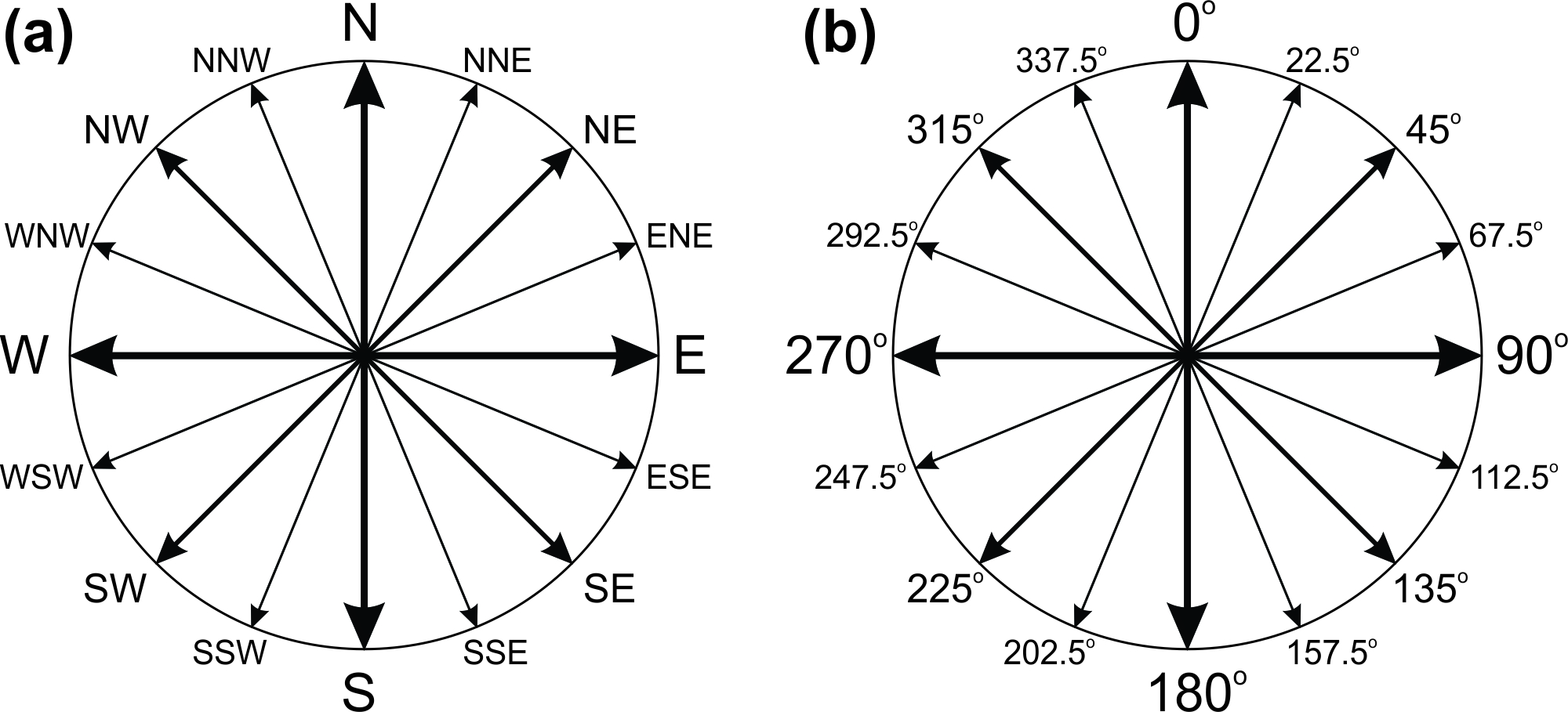
We are all familiar with the points of the compass (Figure 15.1a), also known as cardinal directions. These allow us to specify general directions, but are insufficient to define specific values. For this we use an azimuth, which is the angle measured clockwise from north (Figure 15.1b). The term bearing is often used synonymously with azimuth, although there are also some other uses of the term, so azimuth will primarily be used here. Therefore, north has an azimuth of 0°, northeast is 45°, east is 90°, and so on. The range of azimuth values is 0° to 359°.
Although conceptually simple, defining an azimuth is made a little more problematic because there are three different north arrows to choose from! These are:
- True North: this is the straight-line direction to the Geographic North Pole (GNP). This is also equivalent to following a meridian. An azimuth referenced from True North is called a True Azimuth. Since the GNP is a fixed point on Earth, a True Azimuth for any particular location will never vary.
- Grid North: this is the straight-line direction that runs northwards parallel to the Universal Transverse Mercator (UTM) grid on a NTS map. An azimuth referenced from Grid North is a Grid Azimuth. At most locations, the UTM grid will vary slightly from the latitude-longitude grid, and therefore there is usually a small difference between True North and Grid North.
- Magnetic North: this is the direction towards the North Magnetic Pole (NMP), and is the same direction that a magnetic compass needle points towards. An azimuth referenced from Magnetic North is a Magnetic Azimuth. The Earth's magnetic field is dynamic and always changing its position, and therefore the location of the NMP is always moving. This means that a magnetic azimuth that is correct this year will be slightly incorrect next year. The difference between True North and Magnetic North varies widely.
In reality, the Grid North arrow may be to the west or to the east of the True North arrow and, likewise, the Magnetic North arrow may be to the west or to the east of the True North arrow. All combinations are possible, and are location-dependent.
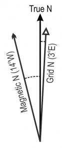
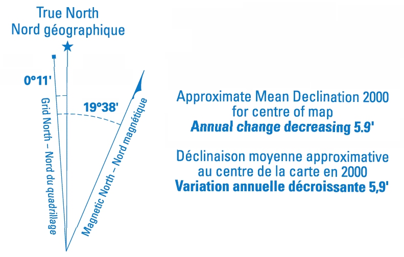
When converting between different types of azimuth, we need to have information about where the three North arrows are —this is typically provided by a declination diagram (although some mapping agencies provide the information verbally). An example is shown on Figure 15.2, using made-up values of True North and Magnetic North:
- The difference between True North and Magnetic North is known as the magnetic declination. In the example shown in Figure 15.2, this is 14° W. We must specify West or East to avoid ambiguity; in this case, it is West because the Magnetic North arrow lies to the west of True North.
- The difference between Grid North and Magnetic North is known as the grid declination. In Figure 15.2, this is 17° W. Again, we must specify West or East to avoid ambiguity; in this case, it is West because the Magnetic North arrow lies to the west of Grid North. Grid declination is necessary when converting between magnetic compass bearings and grid azimuths, which is a very useful field skill.
- The difference between Grid North and True North is known as the grid convergence angle. In Figure 15.2, this is 3° E.
How do we apply this knowledge? Let's apply the grid declination diagram of Figure 15.2 to calculate the azimuths for the direction A-B in Figure 15.3. Assume that the direction from A to B is 75° True. Portraying things visually help us see how the different azimuths can be derived.
- By inspecting Figure 15.3 we can see that the angle between Grid North and the A-B direction is slightly smaller than that between True North and A-B – in fact, it is 3° smaller and therefore: Grid Azimuth = 75° − 3° = 72°.
- Similarly, we can see that the angle between Magnetic North and the A-B direction is 14° larger than that between True North and A-B, so: Magnetic Azimuth = 75° + 14° = 89°.
- So, the direction from A to B can be specified as any or all of: 75° True, 72° Grid, or 89° Magnetic.
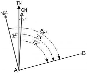
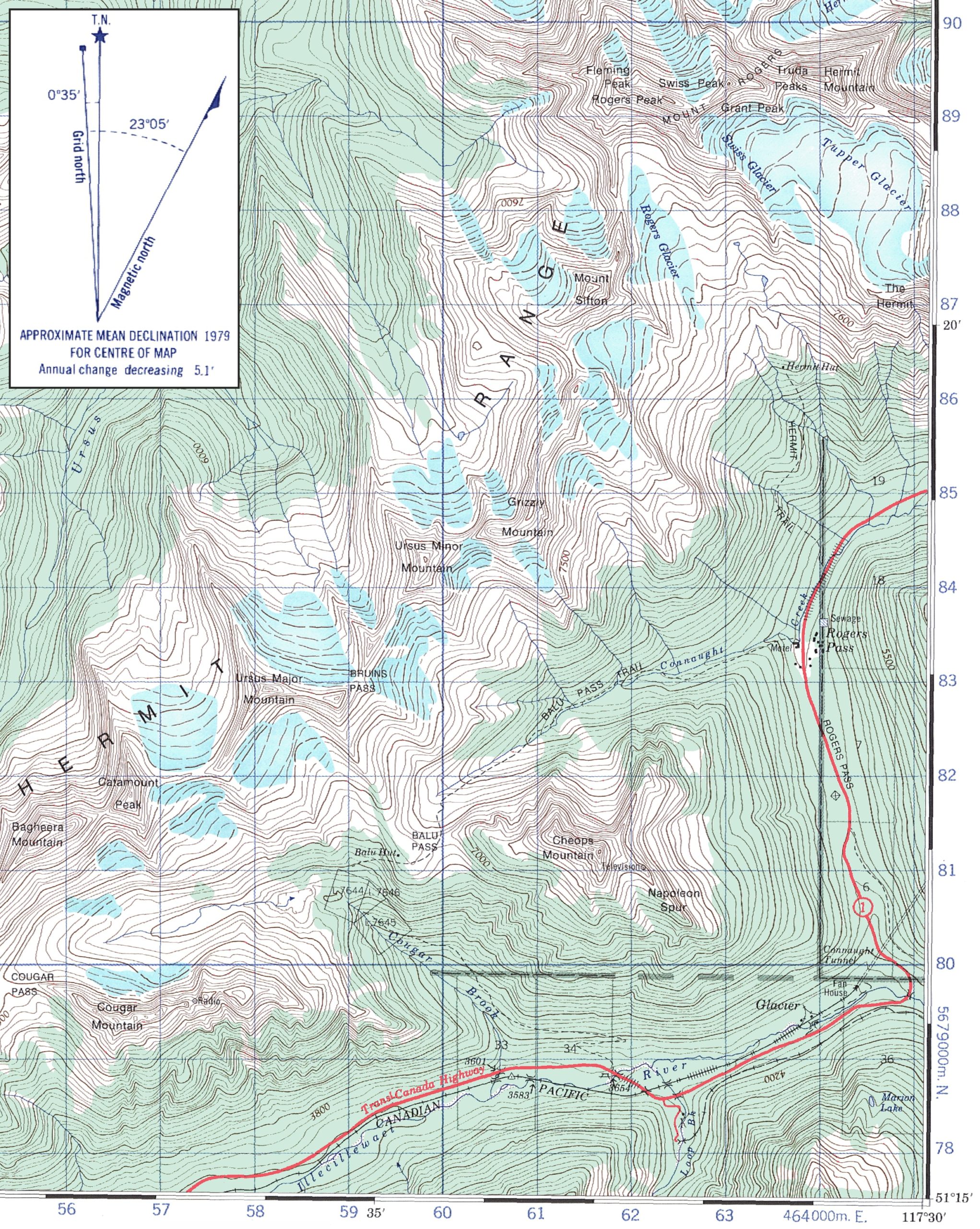
When using azimuths in a real-world situation, we need the actual declination diagrams from the study area (preferably the latest edition). Figure 15.4 and Figure 15.5 show additional examples from Canadian 1:50,000 NTS maps. These diagrams have been simplified for clarity.
Notice that the date of the magnetic information is given, and the rate of change in it. This allows us to calculate the grid declination for the current year. For example, we can see that the grid declination in Victoria, BC, was 19° 38' E in 2000 (Figure 15.4a), and it was decreasing by 5.9' annually. So, in 2020 the value is 19° 38' E minus the accumulated changes in the intervening years. The accumulated changes to the grid declination are the number of years multiplied by the annual change in the grid declination: (2020 − 2000) × 5.9′ = 118′.
Recall that there are 60 minutes in a degree. Therefore, the 2020 value of the grid declination at Victoria is: (Value in 2020 − Accumulated changes = 19° 38′ E − 118′ = 17° 40′ E.
Height Datums and Units
When talking about how high a land surface is, we need a reference level, sometimes referred to as the height datum (not to be confused with a geodetic datum, which is an issue that we don't need to discuss here). Hereafter, we will use the term elevation to define the height above (or, sometimes, below) a height datum. A standard convention in topographic maps is to define elevation relative to the mean sea level (metres above sea level, m a.s.l).
In all cases where elevation is involved, be careful to check what units are being used. The units of elevation are typically feet or metres. See the map's legend to find out. Note that older editions of a particular map sheet might use feet, but later editions of the same map sheet might use metres. Always check!
Spot Heights and Benchmarks
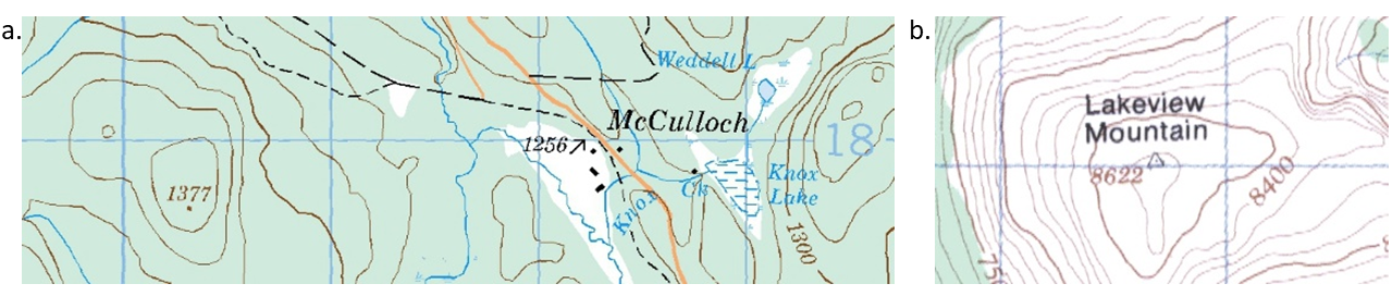
One of the simplest ways to indicate the elevation of land on a map is to use a spot height, which is simply the elevation of a particular point (e.g. the summit of a hill or mountain). Many spot heights are determined from aerial photographs, rather than being surveyed on the ground. Occasionally, you may also see a benchmark shown on a map. These are points that have been surveyed, perhaps as part of construction projects such as highways or rail lines. Locations that have been surveyed for the purposes of map making or town planning (for example) are known as horizontal control points. Many horizontal control points will have a small metal marker affixed to the ground. Figure 15.6a provides examples of a spot height (elevation = 1377, indicated by the brown dot in the centre of a closed contour) and a benchmark (elevation = 1256, indicated by a black arrow). Figure 15.6b shows an example of a horizontal control point (elevation = 8622, indicated by a triangle with a dot in the centre).
Contour Lines
Contour lines (or simply contours) on a topographic map are the most common way of showing the three-dimensional landscape. With practice, a geographer can easily visualize the landscape from a two-dimensional map sheet—a valuable skill.
Contours are lines that connect points of equal elevation. One way of envisaging this is to imagine a valley filled with water. If you drew a line along the shoreline, it would be a contour line. If you dropped the lake level by, say, ten metres and again drew a line along the shoreline you would have a second contour line. Repeating this exercise again and again would leave you with a landscape covered in horizontal lines all ten vertical metres apart (known as the contour interval). You have just made a topographic map! In practice, contours are typically derived by a combination of ground surveys and analyses of aerial photographs.
If we follow the hypothetical procedure for deriving 10-metre contours outlined above, it will be obvious that in very flat areas, a contour interval of ten metres will probably not allow you to pick up the subtleties of the landscape. On the other hand, in a mountainous region a contour interval much greater than ten metres would be advisable, otherwise there would be so many contours that nothing else could be mapped! So, always check the contour interval of the topographic map you’re using. It will normally be found in the map's legend. You will also normally find that contour interval increases as map scale decreases.
A map's contours allow us to derive some fundamental pieces of information: how high we are (our elevation), the steepness (or gradient) of the slope, the slope's profile shape, and the overall relief of the landscape. The usual use of the term relief is to qualitatively describe the range of elevations found in a given area (known as relative relief). A high-relief landscape is one in which there is a great difference between the low and high elevations, such as in mountain ranges. Conversely, a low-relief landscape such as a plateau has little elevation range. Don't confuse relief with elevation. We might have a high-elevation low-relief landscape just as easily as a low-elevation low-relief landscape.
Types of Contours
There are several different types of contours that are good to know about:
- Index contours. Typically, every fifth contour is a bolder line than the regular contour. This is especially useful in high-relief terrain because it allows us to find elevations from the map without having to count every single contour: we can go up/down the mountainside by jumping from one index contour to the next.
- Approximate contours. These are similar to regular and index contours but are drawn using a short-dashed line. This indicates that the exact elevation of the surface was difficult to determine and/or may vary in time.
- Auxiliary contours. If a map shows low-relief terrain adjacent to high-relief terrain, extra contours with a smaller contour interval are sometimes used in the low-relief area to provide more topographic detail. On NTS maps, these are depicted as long-dashed brown lines.
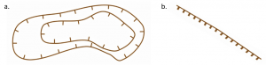
- Depression contours. (Figure 15.7a) These indicate where the land inside a closed-loop contour is lower (i.e., a depression - or hollow - in the surface). The contour line has small hachure marks that face downhill, into the depression.
- Cliff symbol. (Figure 15.7b) Okay, so this is not an actual contour line, but it is worth adding to our list. When slopes get very steep and become cliffs, it may be difficult or impossible to use contours, so a symbol is used instead. The tightly-spaced hachure marks indicate the way the cliff faces.
Interpreting Contour Lines
When interpreting contour lines, there are several key points to remember:
- A contour always separates land that is higher from land that is lower.
- All contours are single, continuous lines. They do not split or cross over each other.
- A closed-loop contour always indicates that there's higher ground inside the loop, unless it is a depression contour.
- On Canadian NTS maps, the convention is that contour labels are oriented to indicate which is uphill. Look carefully at Figure 15.5, for example: along the Illecillewaet River valley at the bottom of the figure, you can see two contour labels on either side of the valley, 3800 and 4200. Uphill is the direction above the top of the number if you were reading it normally.
- If you see contours form a V pattern along a watercourse, the V always points upstream. If you're at a sharp ridge, such as a glacial arete or a large lateral moraine for example, the V pattern in the contours points downhill. Figure 15.5 has several good examples: note the contours along Cougar Brook (at the bottom SW of the figure) where the V pattern points uphill, toward the creek's headwaters. Just to the east of there, examine the contours at Napoleon Spur - the V pattern points down the ridge crest.
Deriving Slope Gradients from Maps
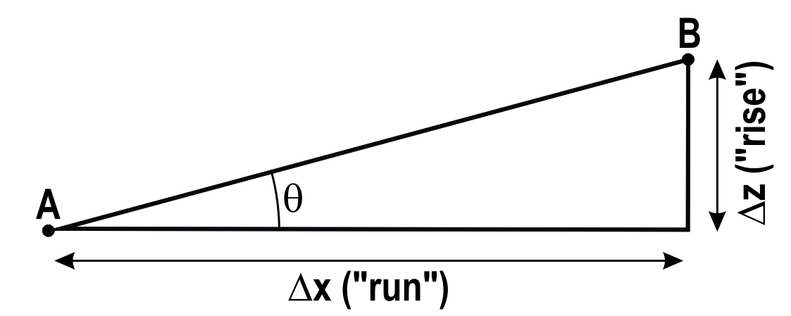
There are several different ways of expressing slope gradient, and all of the most common ones are based on the ratio of horizontal and vertical distances between two points (the classic rise over run situation). To find the slope we need two values: the horizontal distance between points A and B, and the elevation difference between them (Figure 15.8). The horizontal distance (Δx) is found by measuring it on the map and using the map's scale to convert to real-world distance (i.e. exactly what you were doing in Lab 14). The vertical distance between A and B (Δz) is the elevation difference between them, which can be found by interpolating from contours and/or spot heights.
Once we have this information, the slope gradient can be calculated and expressed in three ways:
- As a percent (%): the fraction (rise ÷ run) expressed as a percentage (Equation 15.1):
[latex]\text{Gradient} (\%) = \dfrac{\text{Rise, } \Delta z (m)}{\text{Run, } \Delta x (m)} \times 100\%[/latex]
- As an angle, θ (degrees) (Equation 15.2):
[latex]\text{Gradient} (^{\circ}) = Tan^{-1} \left( \dfrac{\text{Rise, } \Delta z (m)}{\text{Run, } \Delta x (m)} \right)[/latex]
- In elevation change per slope distance (m/km): the gradient expressed with different units used for rise and run, but with the run always reduced to one unit, commonly 1 km (Equation 15.3):
[latex]\text{Gradient}(m/km) = \dfrac{\text{Rise, } \Delta z (m)}{\text{Run, } \Delta x (km)}[/latex]
For example, let us assume that the elevation difference we interpolated between points A and B from contour intervals is 70 m, and the distance measured between A and B is 560m after converting with the map scale. Using the equations presented above, we can express our slope gradient as
- As a percent (%) (Equation 15.1):
[latex]\text{Gradient}(\%) = \dfrac{\text{Rise, } \Delta z (m)}{\text{Run, } \Delta x (m)} \times 100\% = \dfrac{70 m}{560 m} \times 100\% = 12.5\%[/latex]
- As an angle, θ (degrees) (Equation 15.2):
[latex]\text{Gradient} (^{\circ}) = Tan^{-1} \left( \dfrac{\text{Rise, } \Delta z (m)}{\text{Run, } \Delta x (m)} \right) = Tan^{-1} \left( \dfrac{70 m}{560 m} \right) = 7.1^{\circ}[/latex]
- In elevation change per slope distance (m/km) (Equation 15.3):
[latex]\text{Gradient} (m/km) = \dfrac{\text{Rise, } \Delta z (m)}{\text{Run, } \Delta x (km)} = \dfrac{70\text{ m}}{\left( \dfrac{560\text{ m}}{1000\text{ m per km}} \right)} = 125\text{ m/km}[/latex]
If you don't have a calculator with trigonometric functions, you can use an online Arctan Calculator to find the inverse tangent. You will need to divide the rise by the run (70 ÷ 560) as an input for this particular calculator.
Notice that in Figure 15.8 the horizontal distance separating A and B (i.e. Δx) is not the actual ground distance. The true distance from A to B is along the hypotenuse of the triangle in Figure 15.8. For small slope gradients the difference between A-B distance and Δx is negligible, but in steep terrain the A-B distance will be significantly longer than Δx.
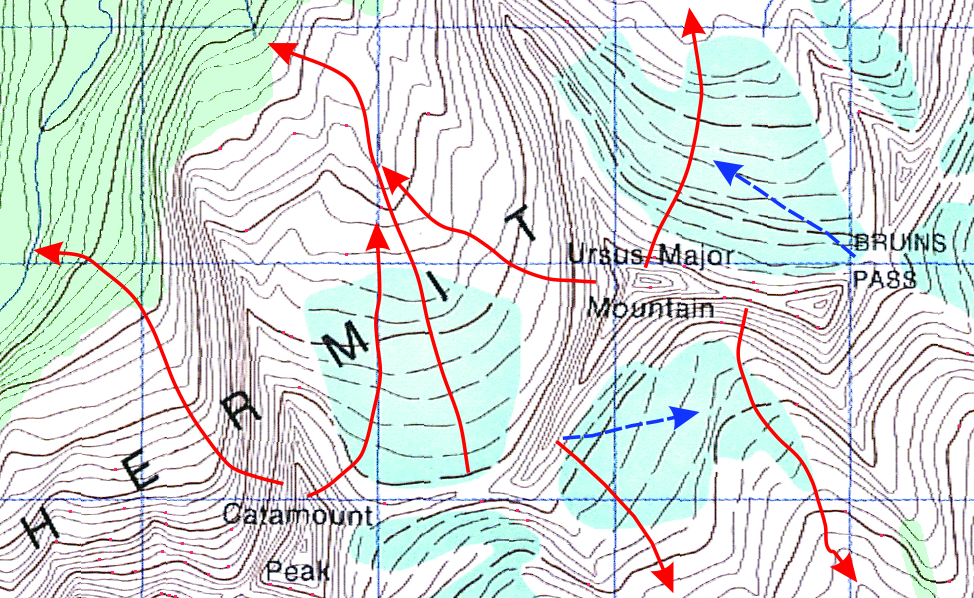
Finally, when deriving slope steepness from a map you must measure Δx along a line that is perpendicular to the contours. This gives the true slope, equivalent to the fall line - think of the direction that water would run down a slope: it would move down the steepest, most direct path, and not deviate along lower-angled routes. In Figure 15.9, true slopes are shown with red arrows. Notice how the red arrows cut across contours at a 90º angle. All other lines crossing the contours represent a false slope (blue arrows), which will always be less than the true slope. On simple slopes, you may be able to measure Δx along a straight line, but realise that the line of true slope will often be curved, as in Figure 15.9.
Topographic Profiles
A topographic profile (Figure 15.10) is a cross-sectional diagram through the landscape, which helps us envisage the nature of the terrain. A profile line might be a simple straight line (which generates a simple profile), or a series of straight lines connected at angles to each other (which generates a compound profile), or more or less any other continuous line, straight or curved. If we used a profile line that cross all of the contours at right-angles, we would have a transverse profile. The longitudinal profile of a river is a transverse profile familiar to geomorphologists and hydrologists.
Topographic profiles are commonly employed to simply show the ups and downs along a particular line (often used in depicting the slopes along a hiking trail). They may also be a bit more complicated like a cross section and show the subsurface geology, such as the way rock strata tilt and/or fold beneath Earth's surface.
It is common to find that topographic profiles are vertically exaggerated (stretched in the vertical direction) to better depict the subtleties of the terrain. Vertical exaggerations of up to about 3x are common; anything more than this tends to make every little bump in the landscape look like hills and mountains!
Vertical exaggeration (VE) is determined as (Equation 15.4):
[latex]\text{VE} = \dfrac{\text{vertical scale}}{\text{horizontal scale}}[/latex]
Vertical Exaggeration Sample Calculation (Try It!)
- A topographic profile is derived directly from a profile line on a 1:50,000 map. What is the horizontal scale?
- Answer: The horizontal scale is 1:50,000.
- The horizontal scale is the same as the map scale.
- The vertical axis of the topographic profile is 5 cm high and represents an elevation range of 1000 m. What's the vertical scale?
- This can be written as 5 cm : 1000 m.Now convert m to cm so the units are the same on either side:There are 100 cm in 1 m, so 1000 x 100 = 100,000 cm. This gives the ratio 5 cm : 100,000 cm.The units are the same on both sides, so they can be dropped, giving 5:100,000.Finally, simplfy the fraction by dividing both sides by 5, to give 1:20,000
- Answer: The vertical scale is 1:20,000
- Using the horizontal and vertical scales, what is the vertical exaggeration?
- Vertical exaggeration = Vertical Scale / Horizontal Scale
- 1/20,000 / 1/50,000 = 2.5
- This means the relative relief seen in the topographic profile is 2.5 times greater than it actually is in reality. The greater the vertical exaggeration, the steeper any given slope appears to be on the profile.
Interpreting the Landscape
The value of topographic maps in allowing us to see the three-dimensional landscape on a two-dimensional map sheet cannot be underestimated. It is a valuable skill, but one that for most people does not come easily. Practice, practice, practice!
Lab Exercises
In this lab you will practice
- Defining direction.
- Interpreting elevation from contour lines.
- Calculating slope gradient.
- Drawing and interpreting topographic profiles.
You will need a calculator, plus an internet connection to download a map and access Google Earth. Some of the exercises may be easier if you are able to print the relevant portion of the map. It is assumed that you have successfully completed Lab 14. It also assumed that you can convert between metres and feet. The exercises should take you 1½ to 3 hours to complete.
EX1: Directions
- Use Figure 15.5.
- Derive the grid declination for the current year using the declination diagram shown in the inset of Figure 15.5.
- Assume that you travel through the Connaught Tunnel, from the SW end to the NE end. On the map, the tunnel is at angle 34° from the UTM grid. Derive all three azimuths. When calculating the magnetic azimuth, use the current year's grid declination that you found in 1(a). Round off all final answers to integers.
- Grid azimuth
- True azimuth
- Magnetic azimuth
- Assume that you are at the motel at Rogers Pass and see an interesting-looking mountain peak but don't know which one it is. You take a compass bearing of 282°. Use this information and your grid declination from 1(a) to determine which mountain peak you are looking at.
EX2: Elevation & Contours
All questions in EX2 refer to Figure 15.5.
- Study Figure 15.5 and determine (use the correct units):
- The contour interval.
- The interval between the index contours.
- Noting that 1 m = 3.281 feet, estimate:
- The elevation (in metres) of Ursus Major Mountain.
- The elevation (in metres) of Rogers Pass.
- Which of the two estimates, Q3a or Q3b, is probably the least accurate? Why?
- Find the Tupper Glacier. The long-dashed lines across the glacier are approximate contours. Why has the cartographer chosen to depict the surface topography of the glacier using this type of contour?
- Find the creek at 585807. It appears to simply stop! No, this is not a cartographic error. What happens to it? Hint: interpret the nearby contour lines.
EX3: Slope Gradients
- Find the average gradient between the historic site at Rogers Pass (the diamond symbol at 642818) and the summit of Mount Cheops at 616812 using Figure 15.5. You can assume that a straight line between these two points is the true slope. Express the slope steepness as:
- A percentage.
- An angle in degrees.
- Elevation change per slope distance.
- The Connaught Tunnel, which carries a rail line beneath Rogers Pass, is about 8080 metres in length. Its northeast portal is at an elevation of 3600 feet (not shown on the map). The southwestern portal is at approximately 644797 on Figure 15.5. What is the average slope of the tunnel? Express it as an angle in degrees correct to two decimal places.
EX4: Topographic Profiles
- Figure 15.11 is a topographic profile of a short hiking trail in the Okanagan region of BC. It is posted at the trailhead so that hikers can see what's in store for them.
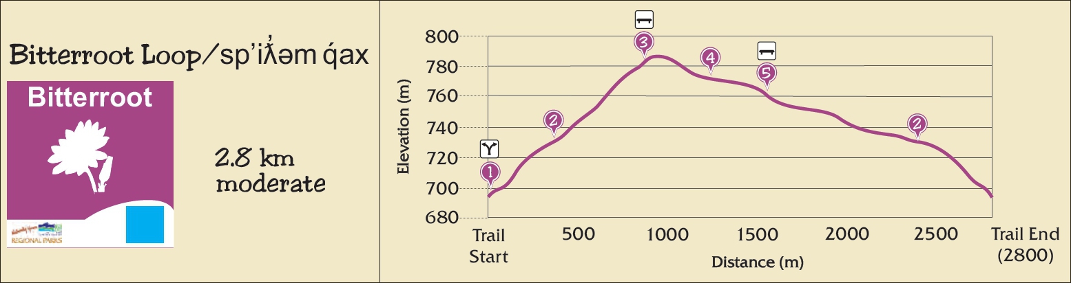
Figure 15.11. Topographic profile of the Bitterroot Loop trail. Source: Rose Valley Regional Park kiosk information, used here with permission from the Regional District of Central Okanagan. [Image description] - The trail looks very steep in places, but this might be due to the vertical exaggeration (VE). Determine the VE to find out. Hint: you can measure the lengths of each axis from the screen and apply the generic scale formula from Lab 14 Map Scales to find the scales of the vertical and horizontal axes.
- Determine the average gradient between point 1 (Trail Start) and point 3 (highest point). Express the slope steepness as
- A percentage
- An angle in degrees
- Elevation change per slope distance
- Now that you have done these calculations, do you think the trail is very steep? Why/why not?
- You have decided to walk across the Illecillewaet River valley shown on Figure 15.5. Your route will take you from Napoleon Spur at 625806 to Marion Lake at 645786 to experience topography first-hand. Although you are prepared for the hike, your friends are concerned that it will be too steep for them.
- Draw a topographic profile on graph paper to convince them they can do it. You will need to print out Figure 15.5, and if you do not have any on hand, graph paper, found in Worksheets. If you require further guidance, please watch these step-by-step video instructions on obtaining data from topographic maps and constructing a topographic profile on graph paper.
- If you were not limited by paper size, how would you alter your cross-section to make it easier to convince your friends to join you?
- What is one advantage of taking a paper map with you on the hike compared to an electronic one?
EX5: Creating Topographic Maps
- Create your own topographic map. As outlined in Contour Lines, contour lines are lines of equal elevation that are interpreted from ground surveys and analyses of satellite images. You have been tasked with creating a topographic map of Acme Creek. Download and print out Map of Spot Heights at Acme Creek found in Worksheets. This document contains spot heights and a graphical scale, and the solid lines already on the map are streams. For further guidance on creating a topographic map from spot heights, please watch this step-by-step video instruction Drawing Contour Lines on a Topographic Map.
- Draw and label contour lines on the map at 25 m intervals between 350 m and 475 m.
- Calculate the scale of the map.
Upload a scan of your complete map as your answer to this question.
Reflection Questions
- Many people rely on their GPS receiver to provide locational and directional information. But GPS receivers can go wrong, or get broken or lost. In 3 - 5 sentences, explain how you would use a map and compass to find your way when the high-tech equipment is no longer an option.
- You want to hike to the top of a mountain but it looks steep and you want to find the easiest (least-steep) route. You open up Google Earth (Web) and know that you can get elevation values for the top of the mountain and a number of points along the base of the mountain. Using the Measure tool for horizontal distances, explain how you could determine the slope of the route options and find the best route?
- A topographic profile is a useful tool for looking at topography of interest. How could you see yourself using this tool outside of this course?
Worksheets
Figure 15.5
Graph paper
Map of Spot Heights at Acme Creek
Supporting Material
How to Find True Slope Along Topographic Profiles
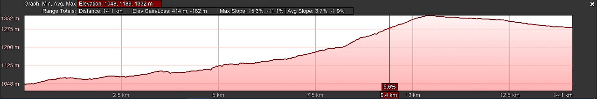
Unless the vertical exaggeration of the profile is 1.0 (i.e. horizontal and vertical scales are the same), slope gradients will not be realistic. They will have to be derived by finding the rise and run of a tangent as shown by the example of a hiking trail in BC on Figure 15.12.
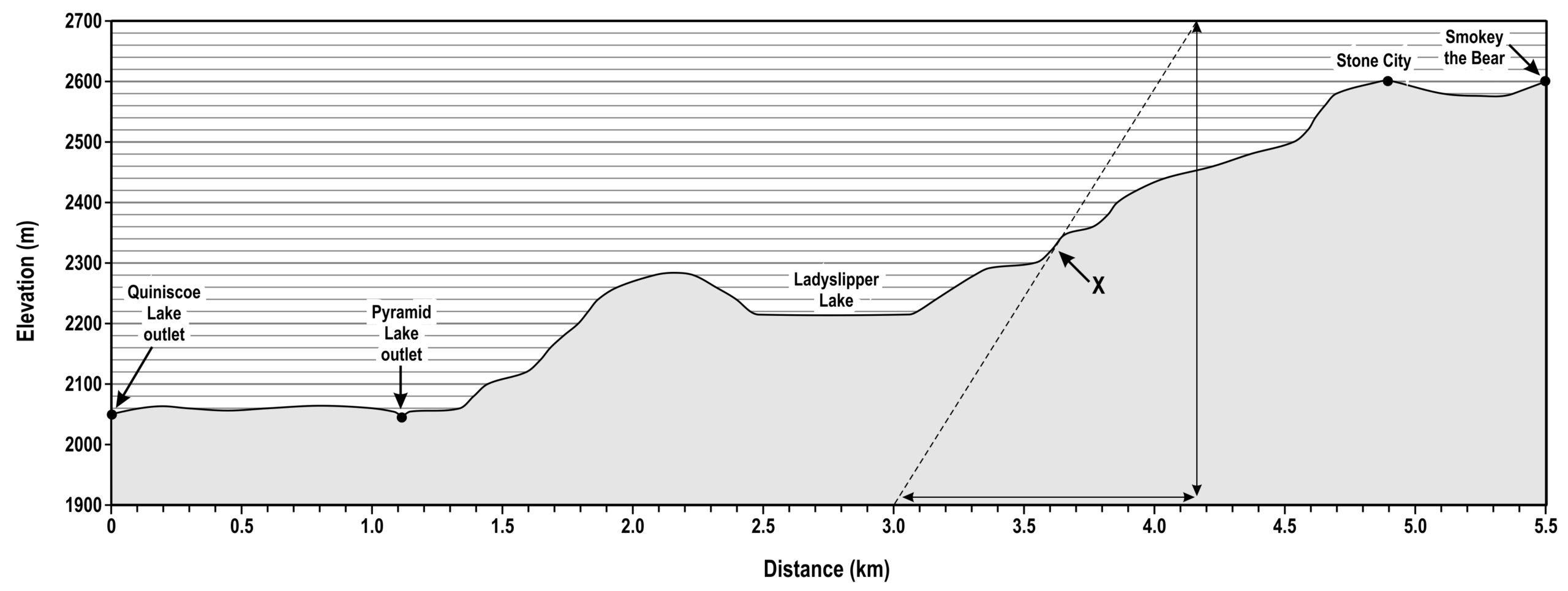
Assume that we want to find the true slope gradient at point X.
Step 1. Draw a tangent through the topographic profile (the sloping dashed line).
Step 2. Find the rise (Δz) and run (Δx) of the line. Here Δz = 800 m and Δx = 1150 m.
Step 3. True slope gradient:
[latex]\text{Gradient} (^{\circ}) = Tan^{-1} \left( \dfrac{\text{Rise, } \Delta z (m)}{\text{Run, } \Delta x (m)} \right) = Tan^{-1} \left( \dfrac{800 m}{1150 m} \right) = 35.0^{\circ}[/latex]
Note how the slope of the dashed-line tangent is much steeper in Figure 15.12 than 35° because of the vertical exaggeration of the profile.
Downloading NTS Topographic Maps
Option 1: If you don't know the map sheet's number. Access the GeoGratis Topographic Information website and select the Geospatial Product Index - HTML. You can then zoom in or out of the map and the map codes will appear. For example, zoom in on Vancouver. You will first see 92 appear, then a grid with letter codes, and then number-letter-number codes which are the 1:50,000 map IDs; downtown Vancouver is map sheet 92G06. You may get access to the maps directly from here, but if not, record the map sheet number and go to Option 2.
Option 2: If you know the map sheet's number. Use GeoGratis's ftp site for 1:50,000 map sheets. You will probably find that the canmatrix_geotiff versions are the easiest to use. Alternatively, *.tif and *.pdf files are also available. These are all scanned versions of the original NTS map sheets.
Image Description
Figure 15.8. Fundamental elements of a slope.
A schematic diagram that represents a hillslope with a right-angle triangle. The components necessary to calculate the slope gradient between the lowest point, Point A, and the highest point, Point B are also identified. The line from Point A to Point B is the hypotenuse of the triangle. This is the line for which the slope gradient is to be calculated. The slope gradient is calculated by measuring the horizontal distance between Point A and Point B (delta x), which is also known as the “run”, and the vertical difference between Point A and Point B, or elevation change (delta z) which is also known as the “rise”. The right-angle of the triangle is formed where lines drawn horizontally from Point A and vertically from Point B connect. The slope gradient can also be expressed as an angle, theta, the angle between the horizontal line and the slope of interest.
Figure 15.11. Topographic profile of the Bitterroot Loop trail.
An example of a trail map that may be found at a trailhead. The left panel of the image is the name of the trail in English and nsyilxcen, and the distance and difficulty of the trail. The Bitterroot Loop is 2.8 kilometres long and of moderate difficulty. The right panel is a topographic map that depicts the change in elevation along the length of the trail. Elevation in metres is on the y axis and distance along the trail in metres is on the x axis. The trail starts and finishes approximately 695 m in elevation and rises to 785 m elevation over a total distance of 2800 m.
