Canada has the longest shoreline of any country in the world, but estimates of how long the shoreline actually is will vary greatly depending on how it is measured. In British Columbia, for instance, the straight-line distance between Vancouver and Prince Rupert is approximately 800 km, but the length of the coastline between the two cities is about 41,000 km when traced on a relatively detailed map.

Waves are the dominant energy source on exposed, open-ocean coasts, and when wave energy is expended on the shoreline, there is the potential for rapid and significant geomorphic change. An understanding of coastal geomorphic processes and landforms is important not only for pure scientific interests but also to avoid potentially disastrous consequences of the human occupation and use of coasts.

Pre-Readings

The Littoral Zone

Fundamental to coastal geomorphology is an understanding of the littoral zone. The littoral zone includes the coast, beach, nearshore environment, and a part of the offshore environment. This lab concerns itself with the processes that occur in this zone, and the resulting landforms created by erosion, transport and deposition.

Properties of Waves

The source of energy for most coastal erosion and sediment transport is wave action. Waves are distortions of the still water surface that contain (a) potential energy by virtue of water molecules being displace above and below the still water line; and (b) kinetic energy by virtue of water molecules being in motion. The faster the wind and the longer the fetch (or distance of open water across which the wind blows and waves travel), the larger the waves. Large waves have much greater energy than smaller waves, in fact, wave energy is proportional to the wave height squared.

It is important to realize that waves in the open ocean (referred to as deep water waves) do not move the water forward, but rather the water molecules move in circular orbits. If you have ever floated offshore in a small boat or inner tube you will know this to be true; a moving wave will pass beneath the boat and cause you to rise and fall but you will not move any appreciable horizontal distance forward or backward. The situation is different close to shore where there is net movement of the water in the direction of wave propagation, but where there can also be currents (e.g., longshore, rips). Waves are described using basic measurements such as wave height, wavelength (Figure 23.1), and wave period.

Wavelength is defined as the horizontal distance from wave crest to wave crest (or trough to trough), while height is the vertical distance between the trough and crest. Both values are commonly measured in metres (m). Open ocean waves are modelled as a sinusoidal curve, with symmetry above and below the still water level. The time taken for successive crests to pass a fixed point is called the wave period, measured in units of time such as seconds (s). One of the interesting aspects of wave motion is that the period remains essentially constant despite changes in the wave form as it enters shallow water.

The velocity or phase speed of the wave, V, can be calculated if the wavelength, L, and the wave period, P, are known (Equation 23.1):

Equation 23.1.

[latex]V = \dfrac{L}{P}[/latex]

Given that wavelength is commonly measured in metres (m) and wave period in seconds (s), the units of wave velocity are metres per second (m/s).

For example, let us assume that a wave has a wavelength of 16 m and a wave period of 4 s. The velocity (V) of the wave may be calculated using Equation 23.1 as:

[latex]V (m/s) = \dfrac{L (m)}{P (s)}[/latex]

[latex]V (m/s) = \dfrac{16m}{4s} = 4\text{ m/s}[/latex]

This relationship can be re-arranged to solve for wavelength or wave period. A good way to think about how the equation can be re-arranged is by examining the units of the output and making sure they make physical sense to you. For more detailed explanations, please refer to SERC Carleton’s How do I calculate rates? Calculating changes through time in the geosciences and How do I isolate x (or P or T …) in a formula? Rearranging equations to solve for a given variable.

Long period waves (referred to as long waves or swell waves) travel faster than short, locally-generated sea waves. As a consequence, waves have a tendency to sort themselves out as they move away from the storm centre that generates wave motion in the open ocean. Long swell waves that have travelled hundreds of kilometres may have periods of up to 15 seconds. Smaller waves have periods of only a few seconds.

Wave Refraction

In much the same manner as light is refracted (bent) through a prism, waves are subject to refraction or bending of the wave crests as they approach the shore. Whenever waves approach a shoreline at an oblique angle, the presence of the sea floor turns the waves to become more parallel to the shore. The reason is that the offshore portions of the wave crest are not influenced by the bottom and are free to travel at their optimal speed (i.e., their deep-water velocity). In contrast, the onshore portions of the wave crest are impeded by the presence of the bottom and therefore are forced to slow down.

On an indented coast the situation is more complex, but Figure 23.2 below shows what is expected to happen. The wave crests in deep water approach the shore perpendicular to the general trend of the coast. The wave crests approaching the headlands begin to be affected by the sea floor first, when they are just under a kilometre from the shore. These portions of the wave crests slow down, shorten in wavelength, and increase in height. The same crest approaching the bay continues unimpeded (because water depth in front of the bay is deeper) and so moves ahead of the wave segment at the headland. At position 1 on Figure 23.2 Segments A and B are in deep water and are unchanged, but by the time they have reached position 3, A has slowed down and shortened its wavelength. It therefore lags behind B which is still unchanged. By the time the wave reaches position 4 on Figure 23.2, A is about to break on the headland while B is advancing more slowly into the bay. The end result is that the wave crest is bent progressively by refraction so as to conform to the bathymetric contours and ultimately break parallel to the shoreline.

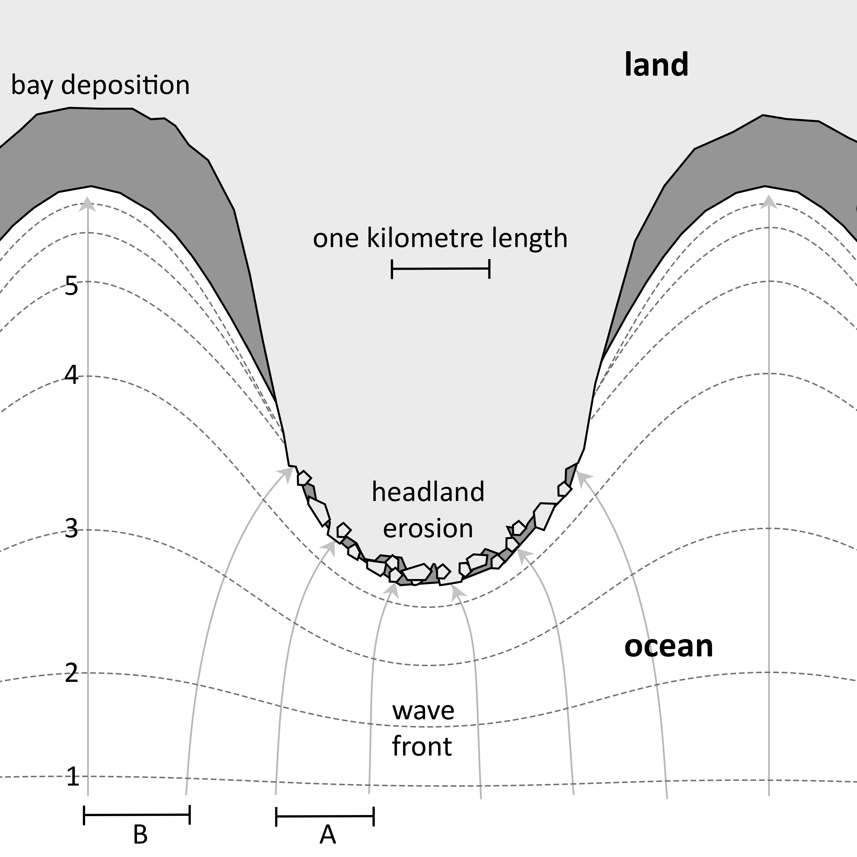
The convergent pattern of the orthogonals show the direction of movement of the wave crest (the solid lines drawn at right angles to the wave crests with arrow tips). The closer spacing of the orthogonals near the headlands show how the wave energy in segment A is concentrated onto the headland. In the bay, wave height is reduced since the energy of segment B is spread out across a greater length of shoreline (orthogonals are further apart). Therefore, headlands tend to be sites of erosion while bays tend to be sites of deposition. The tendency is for waves to create a smooth, linear coastline, but this often does not happen because of differences in the strength of rocks (resistance to erosion) on headlands versus embayments.

Erosion, Transportation and Deposition Along Coasts

A number of mechanical and chemical effects produce erosion of rocky shorelines by waves. The types of erosional landforms that result depend on the geology of the coastline, the nature of wave attack, the tidal regime, and long-term Sea Level Change. Examples of erosional landforms include wave-cut notches, marine cliffs, sea caves, arches and sea stacks.

Transportation by waves and currents is necessary to move rock particles eroded from one part of a coastline to a place of deposition elsewhere. One of the most important transport mechanisms results from an oblique angle of wave attack relative to the shoreline orientation. The upward movement of water onto the beach (swash) occurs at an oblique angle. However, the return of water (backwash) is at right angles to the beach, resulting in the net movement of beach material laterally. This movement is known as beach drift. Waves approaching the shoreline at an oblique angle also force longshore currents, especially in troughs between nearshore sand bars. The combination of longshore currents with the never-ending cycle of swash and backwash is called longshore drift or littoral drift and can be observed on all sandy beaches.

In addition, tidal currents along coasts can be effective in moving eroded material. While incoming and outgoing tides produce currents in opposite directions on a daily basis, the current in one direction is usually stronger than in the other, resulting in a net one-way transport of sediment. Longshore currents and tidal currents in combination with waves will determine the net direction of sediment transport and ultimately where sediment is eroded and deposited along the shoreline.

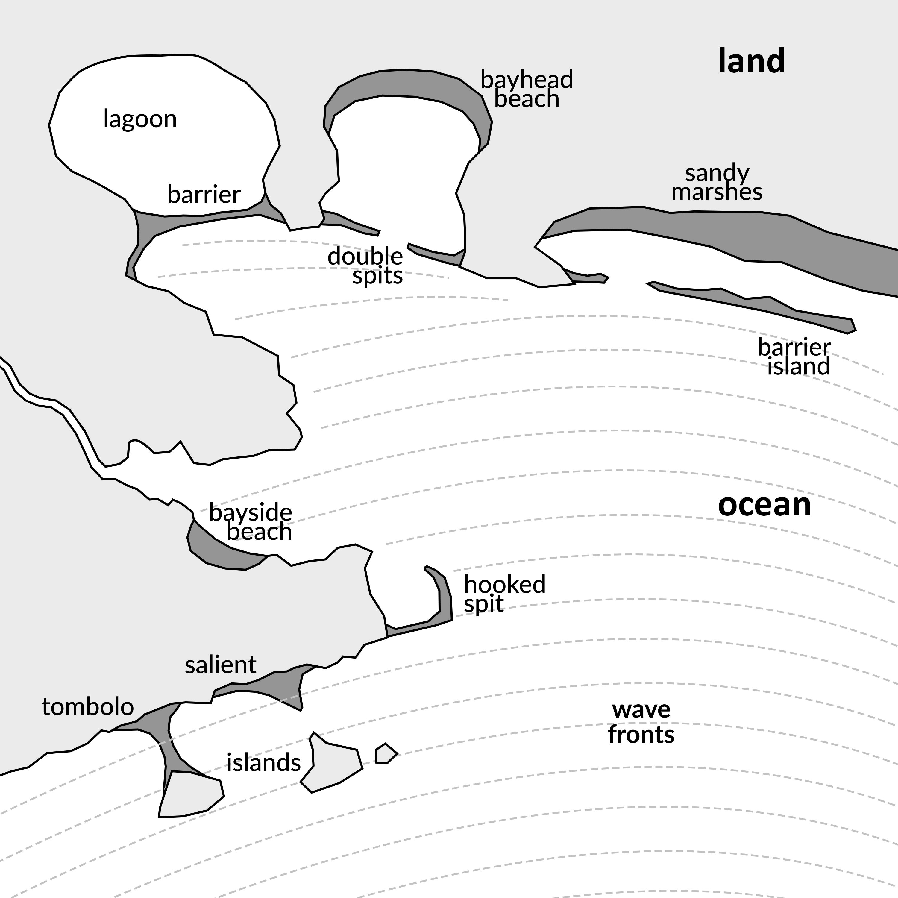
Many kinds of depositional landforms are possible along coasts depending on the geological configuration of the coastline, direction of sediment transport, character of the waves, and shape and steepness of the underwater slope offshore. Some common depositional forms are spits, bayhead beaches, barrier beaches or islands, tombolos, hooked spits, salients, bayside beaches, lagoons, and sandy marshes (Figure 23.3).

When specifying the direction of coastal sediment transport, we specify the direction that sediment is moving towards. For example, if sediment is moving from Los Angeles, USA, to Vancouver, Canada, then the direction it is moving is north. Cardinal directions are the points on the compass used to specify general direction, and include north (N), south (S), east (E) and west (W), and their derivatives. For further details, refer to Lab 15 Directions.

Coastal Sediment Budgets

Coastal sediment budgets are used to understand changes in beaches and coastlines over time. When constructing a sediment budget, a geomorphologist will try to quantify (measure or estimate) the inputs, outputs and changes in storage within a coastal compartment referred to as a littoral cell. The concept of a littoral cell is to a coastal geomorphologist what a watershed or drainage basin is to a hydrologist – it is an easily identified system of study with natural boundaries.

For a beach system, the sediment budget is generally concerned with sand-sized particles (0.2 – 2 millimetre (mm) diameter) and larger (> 2 mm diameter). The inputs and outputs of a beach sediment budget may consist of some or all of the components listed in Table 23.1. It is important to note that there are a number of locations/processes that can act as sources or sinks of sediment, depending on the local geography and time period of interest. This explain why coastal dunes are listed as inputs and outputs: the dune may contribute sediment to the beach (input) or be built up by sand transported from the beach (output). Inputs can come in the form of point sources (e.g., river) or line sources (e.g., cliff erosion).

Inputs and outputs are commonly expressed as volumetric rates of sediment movement (e.g., cubic metres per year, m³/y).

When inputs are greater than outputs over some period of time, a beach will grow (prograde, storage is positive). When outputs are greater than inputs, the beach will shrink (erode, storage is negative). What will happen when inputs equal outputs? That’s correct, the beach will stay the same size. The net sediment budget is equivalent to the change in storage and is (Equation 23.2):

Equation 23.2

ΔStorage = Inputs – Outputs

For example, let us assume that each year Bondi Beach receives 70,000 m³/y of sand from littoral drift and 5,000 m³/y from coastal dunes, and loses 79,000 m³/y of sand to littoral drift. The net sediment budget is (Equation 23.2):

ΔStorage = Inputs − Outputs

ΔStorage (m³/y) = ( 70,000 m³/y + 5,000 m³/y) − ( 79,000 m³/y)

ΔStorage (m³/y) = 75,000 m³/y − 79,000 m³/y

ΔStorage  (m³/y) = − 4,000 m³/y

Because the change in storage is negative, this calculation indicates that Bondi Beach is shrinking at a rate of 4,000 m³/y. Don’t worry, this calculation is fictional. The beach will still be there when you finally make it to check out the location of Bondi Rescue. When solving this equation, remember your order of operations. First add all the components inside the brackets and then subtract the outputs.

Note that the units we are using are a rate, just as velocity is a rate. This means that this relationship can be rearranged to solve for volume of sand or time, depending on which variables are known.

Sea Level Change

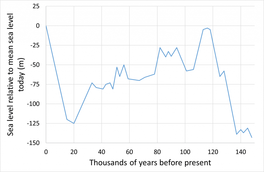
Sea level is not constant through time or space. When sea level falls, the coastline moves in an oceanward direction. When sea level rises, the coastline moves in a landward direction. Figure 23.4 shows changes in global sea level over the past 150,000 years.

A number of processes contribute to changes in sea level both globally and locally:

• Growth and decay of glaciers and ice sheets affect the amount of liquid water.
• Land surface elevations change through time due to plate tectonics.
• Local land surface elevation changes due to melting of overlying glaciers (isostatic adjustment).
• Rise or fall of water level due to heating and cooling of water that leads to expansion and contraction of water in terms of total volume in the oceans.

Bathymetric maps show the topography (depth) of the land surface below the water level in the same way that a topographic map shows the topography (elevation) of hills and mountains. On bathymetric maps, contour lines connect points of equal depth below present sea level.

Lab Exercises

This lab includes a number of exercises to help build your understanding of coastal processes. In this lab you will:

• Calculate wave characteristics based on different types of input data.
• Identify the direction and source of coastal sediment transport from satellite imagery.
• Identify coastal landforms from satellite imagery.
• Calculate coastal sediment budgets.
• Interpret sea level change from graphs and depict spatially on a map.

You will need access to Google Earth (Web) and Google Earth Engine Timelapse. If you wish to complete mapping exercises by hand, you will also need the ability to scan or photograph an image and create a PDF. These exercises will take 2-2.5 hours to complete. Submit your work following the instructions of your professor or lab instructor.

EX2: Coastal Sediment Transport

Figure 23.5 shows James Island, which is located off the east coast of Vancouver Island, BC.

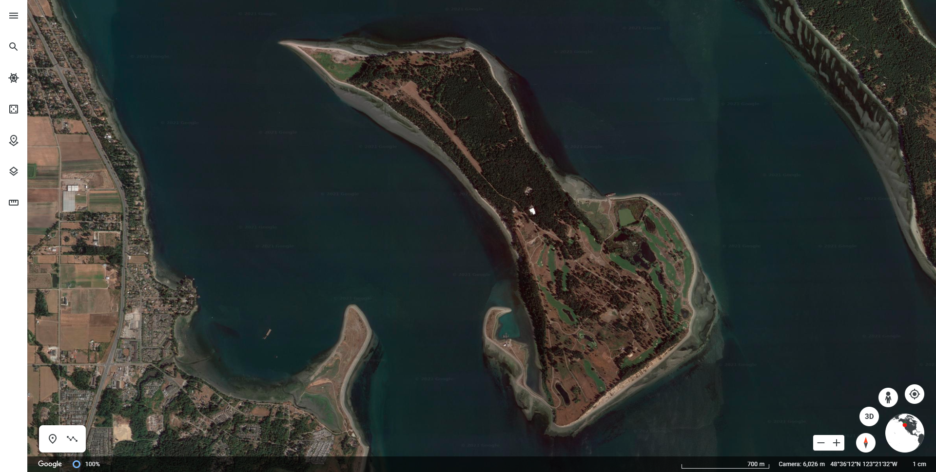
3. What is the cardinal direction of coastal sediment transport on James Island (Figure 23.5)? What evidence leads you to that conclusion?
4. What is the source of the sediment being moved along the coast? Open Google Earth (Web) and enter the coordinates provided in the caption of Figure 23.5 to have a closer look around James Island.
5. View the Google Earth Engine Timelapse for the spit at 34.63095°, -76.47419°. What is the cardinal direction of longshore drift?

EX3: Coastal Landforms

Figure 23.6 shows a number of coastal landforms near Tofino, BC.

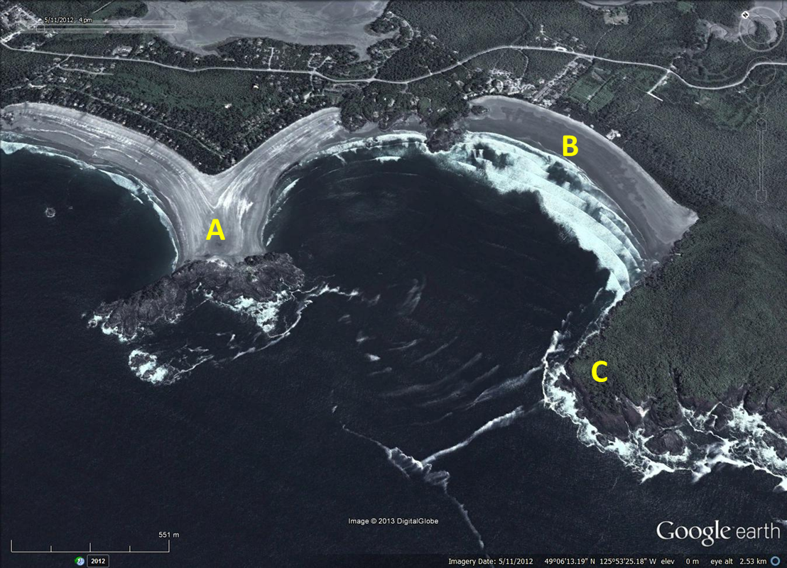
6. Identify the coastal landforms labelled A, B, and C on Figure 23.6.
7. Explain how feature A likely formed.
8. What is the dominant direction of incoming waves on Figure 23.6? What is your evidence for this?
9. Locate the following features on Google Earth (Web) by copying and pasting the coordinates or name into the Search tool (magnifying glass icon, second from top in list on left of screen). Answer the associated questions.
   1. 21°19’59”N, 158°07’25”W.
      1. Are these natural or artificial bays? How can you tell?
      2. What geomorphic role do the little islands play at the mouth of the bays?
   2. 21°16’24”N, 157°49’29”W.
      1. What are these features?
      2. What purpose do they serve?
   3. The islands of Bora Bora and Tahaa, French Polynesia.
      1. What type of coastal landform are these features?
      2. Which island is older? Explain your evidence for this.
      3. What will they eventually become?

EX4: Beach Sediment Budgets

A sediment budget was developed for Sandy Beach in the 1960s. Figure 23.7 is a schematic of the area and includes the boundary of the littoral cell (dashed line) and inputs and outputs.

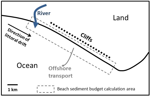
Volumetric rates of inputs and outputs are provided in Table 23.2.

Table 23.2. Sandy Beach sediment budget.

Inputs	Sand volume (m3/y)
Littoral drift	5,000
Sandy River	123,000
Cliff erosion	42,000
Outputs	Sand volume (m3/y)
Littoral drift	145,000
Offshore transport	18,000

10. Based on the data in Table 23.2, calculate the net sediment budget in the 1960s. Show your work.
11. During the 1960s, was the beach growing, shrinking or staying the same?

In the 1970s and 1980s a number of multi-millionaires built mansions on the top of the cliffs above the beach. The owners were worried about their homes falling into the ocean due to erosion of the cliffs, and constructed revetments along the cliff base. As a consequence, cliff erosion was reduced to 20,000 m³/y. Erosion wasn’t completely stopped because a section of the cliff was managed by a Coastal Conservancy that did not want to build revetments. Thus, certain portions of the cliff remained natural and unprotected.

12. It is now the year 2021, and the effects of the decrease in cliff erosion are starting to become evident.
    1. Re-calculate the net sediment budget considering the change in cliff erosion. Show your work.
    2. Is the beach now growing, shrinking, or staying the same?
    3. Will erosion or deposition be uniformly distributed along the entire length of shoreline backed by the cliff? Explain.

Changes in the sediment budget affect the width of the beach (beach distance from cliffs to sea level) over a period of years to decades. A coastal engineer has predicted that a positive sediment budget of 5,000 m³/y would add 0.1 m to the width of the beach, while a loss of 5,000 m³/y results in a decrease of 0.1 m to the width of the beach.

13. Assume that the beach had an average width of 35 m prior to the construction of the revetments. How long did it/will it take for the beach to recede (erode) back to the base of the cliff? Hint: Use the net sediment budget you calculated in Q12a.

Worksheets

Back to EX6

Shoreline Bathymetric Map

• Shoreline Bathymetric Map [PNG]
• Shoreline Bathymetric Map [WORD]
• Shoreline Bathymetric Map [ODT]
• Shoreline Bathymetric Map [PDF]

References

Davidson-Arnott, R., Bauer, B., & Houser, C. (2019). Introduction to Coastal Processes and Geomorphology (2nd ed.). Cambridge University Press, New York, NY.

Shackleton, N.J. (1987). Oxygen isotopes, ice volume and sea level. Quaternary Science Reviews, 6(3-4), 183-190.