Lab 14: Map Skills I – Defining Location
Ian Saunders; Chani Welch; and Saoirse MacKinnon
Maps represent one of the most important tools that geographers use to communicate information about the spatial associations of the phenomena which they study. We can think of maps as being models, in the sense that they typically aim to reduce the complexity of the real world into something that can be studied more easily. There is a bewildering array of map types; common map types are base maps, which show the essential features of the landscape, and thematic maps, which show the spatial distributions of probably any geographic variable you care to think of. In Canada, base mapping at the federal government level is referred to as the National Topographic System (NTS).
This lab is largely about how to use NTS maps, plus some Google Earth (Web) practice, to address fundamental questions that geographers ask: How can we specify where a place is? (Geographers know where it’s at!) How far is it between two places?
Learning Objectives
After completion of this lab, you will be able to
- Use geographical coordinates and Universal Transverse Mercator (UTM) coordinates to specify locations.
- Convert between different units of geographical coordinates.
- Understand the applications of map scales.
- Derive distances and areas from a map.
- Use Google Earth (Web) to derive coordinates and distances.
Pre-Readings
Geographical Coordinates
The term geographical coordinate refers to the latitude-longitude system, which defines a location using angles measured from some prescribed baseline. Latitude is the angle measured north or south from the equatorial plane to your position. Lines of equal latitude form parallels that run west-east. The Equator is at latitude 0°. Latitude ranges from 90°S (South Pole) to 90°N (North Pole). When using latitude data in purely numerical form (i.e. the N or S isn’t specified), northern hemisphere data are considered as positive and southern hemisphere data negative. Unless you’re using purely numerical data, you must specify N or S to avoid ambiguity.
Since parallels must, by definition, be parallel (go figure!) each line of latitude must have a fixed north-south separation between them. On Earth’s surface, one degree of latitude represents a distance of approximately 111 km. This is a useful thing to remember, because it enables you to estimate the north-south distance between two places if you know their latitudes. For example, the northern boundary of British Columbia is the 60°N parallel, and most of the southern boundary is at the 49th parallel (i.e. 49°N); therefore, a very quick estimate of the distance between the two boundaries is:
(60 – 49) × 111km = 1221 km.
Longitude is the angle measured west or east from the Prime Meridian (or Greenwich Meridian, since it runs through the observatory at Greenwich, England) to your position. Lines of equal longitude form meridians that run north-south from the North Pole to the South Pole. This means they are not parallel: they are farthest apart at the Equator and converge towards the poles. The Prime Meridian is at longitude 0°. Longitude ranges from 180°W to 180°E. When using longitude data in purely numerical form (i.e. the W or E isn’t specified), eastern hemisphere data are usually considered as positive and western hemisphere data negative (but beware – occasionally you may come across the reverse of this convention, for example when using online distance calculators; you need to stay sharp!). Unless you’re using purely numerical data, you must specify W or E to avoid ambiguity. Note that the 180°W meridian is also exactly the same as the 180°E meridian, and is also the general location of the International Date Line.
The distance between individual meridians is approximately 111 km at the Equator (i.e. same distance as one degree of latitude) and decreases as you get closer to the poles; this means that estimating west-east distances from longitude data is a little trickier than it is with latitude. The simple solution is that the surface distance between two meridians, one degree of longitude apart, is: 111km × cos(LAT), where LAT is your latitude. For example, the west-east distance for one degree of longitude in the central area of British Columbia (55°N assumed) is:
111km × cos(55) ≈ 64 km.
Geographical coordinates are based on angles, and there are two common ways to express these:
- In decimal degrees (DD). Here are three examples: (i) 50.6°N; (ii) 50.57°N; (iii) 50.56789°N. Obviously, the more decimal places we use, the greater the implied accuracy of the coordinate. Using coordinate (i) would be appropriate when defining the location of a town, for example, because this only requires an approximate value. But if we wanted to define the location of a particular building in that town, then greater precision is required, and the extra decimal places in coordinate (iii) would be needed.
- Using a sexagesimal system, which divides one degree into sixty minutes and one minute into sixty seconds. Here are three examples, exactly the same as those in (a), above: (i) 50° 36' N; (ii) 50 34' 12" °N; (iii) 50 34' 04.404" °N. Notice here that if we want to specify very precise locations using the sexagesimal system, we have to add decimal places to the seconds. The units of this system are degrees, minutes and seconds, and hence the units of this system are commonly abbreviated to DMS.
Geographical Coordinates on Maps
Different mapping agencies use different ways to denote geographical coordinates on maps, but a common method is to show latitude and longitude markers around the margins. On Canadian 1:50,000 NTS maps (e.g., Figure 14.1), the alternating black and white bar lines along the margins represent minutes of latitude (vertical lines) and longitude (horizontal lines). The latitude increases as one moves northwards (up) away from the Equator and longitude increases as one moves westwards (left) away from the prime meridian. It might also be useful to note that the neatlines (i.e. the actual edge of the map) of NTS maps are defined by parallels and meridians (i.e. the top and bottom edges run exactly west-to-east, and the sides run exactly north-to-south).
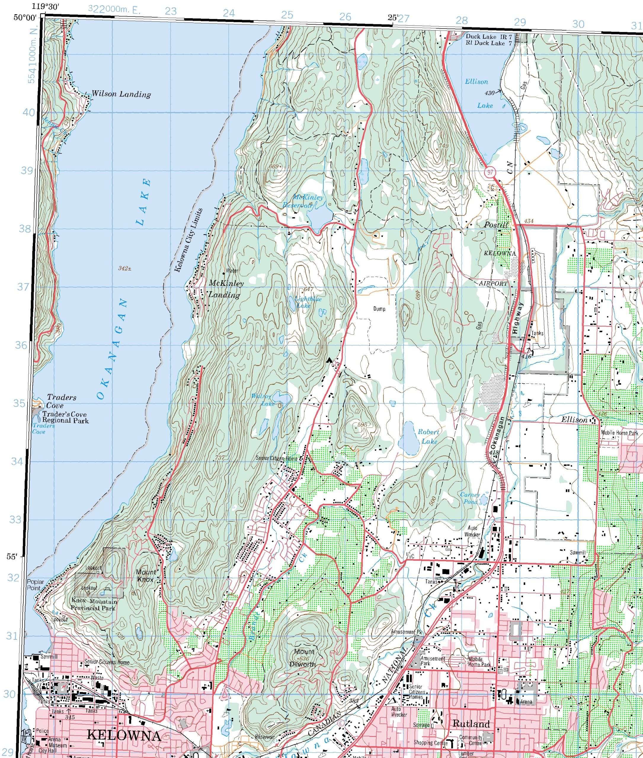
There are several items to note in Figure 14.1:
- The marginal information related to geographical coordinates is in black and white:
- black and white bars up the side: there are seven of them, each representing one minute of latitude, and therefore the north-south extent of the map shown here is nearly 7 minutes of latitude. Every fifth minute has a label: notice the 55' marker in the lower-left edge of the map.
- black and white bars along the top margin each represent one minute of longitude, and therefore the west-east extent of the map shown here is about 8½ minutes of longitude.
- The northwest corner of the map has coordinates of 50°00' and 119°30', but we are not told which hemispheres. The map-makers assume that we know that Canada is in the northern and western hemispheres.
- Values of latitude increase bottom-to-top, because we are moving farther away from the Equatorial plane. Values of longitude increase right-to-left, because we are moving farther away from the Prime Meridian.
For instructions on how to determine the geographical coordinates of a location when using a NTS map, refer to the Supporting Material.
UTM Coordinates and Grid References
The Universal Transverse Mercator (UTM) coordinate system is a type of Cartesian system, which means that a location is specified using a rectangular grid. You will be familiar with simple graphing using an x-axis and a y-axis, in which a point can be located by its x value and y value, as follows: (x,y). The UTM coordinate system is similar, but bigger, since it covers most of the Earth! UTM doesn’t extend to the polar regions; there a separate system, the Universal Polar Stereographic (UPS) system, applies. Common mapping software (e.g., Google Earth) and GPS receivers often use full UTM coordinates, so it’s important to understand how they work.
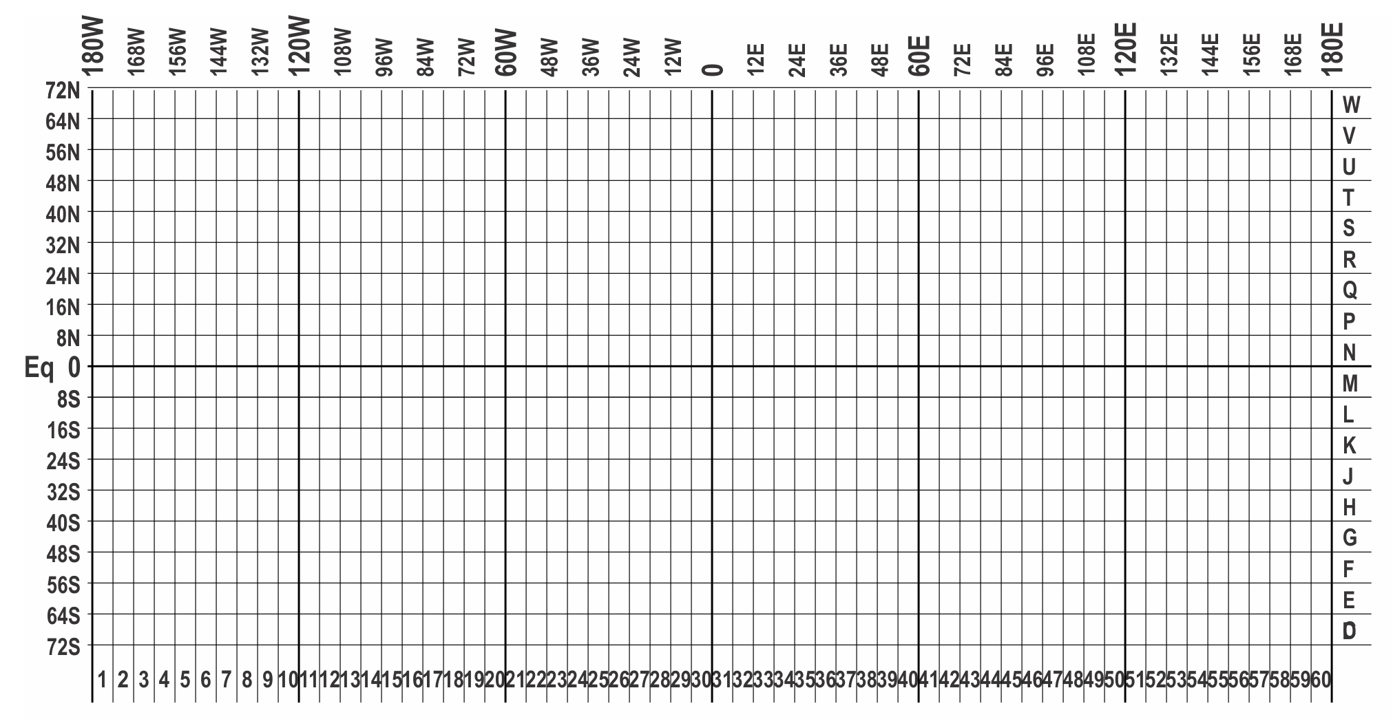
The UTM system divides the Earth into sixty identical north-south strips or UTM zones, each 6 degrees of longitude wide and identified by a number (Figure 14.2). Each zone has a central meridian down the middle. Zone 1 is 180°W-174°W, Zone 2 is 174°W-168°W, and so on. So, for example, we find that British Columbia falls into zones 7 to 11. Each zone has latitudinal divisions 8° latitude in extent, that have letter designations (with I and O being excluded) starting with C at 80-72°S. The Equator is the boundary between M and N (useful to remember because the letter indicates which hemisphere you’re in: C to M are southern and N to X are northern).
So, with a simple number-letter combination we can easily specify any of the squares (or UTM quadrilaterals as they're more formally known) shown on Figure 14.2. This is useful information, of course, because it immediately gives us a good idea of where we are.
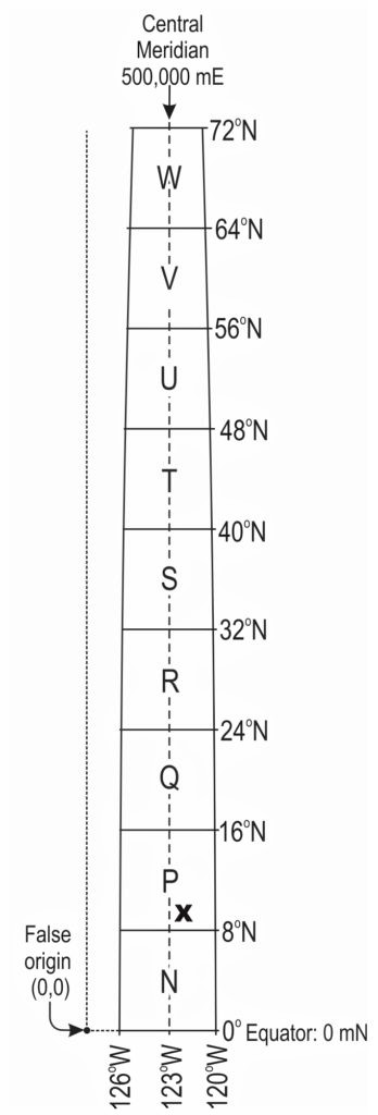
In each of the northern and southern hemispheres, the UTM zone is treated as a very large (x,y) grid. All zones have a false origin (0,0) from which the x value (the easting) and the y value (the northing) are derived (Figure 14.3). This is placed 500,000 m west of the zone’s central meridian, forcing all eastings to be positive (UTM has no negative numbers). In the northern hemisphere, the false origin is at the Equator; in the southern hemisphere it is set at 10,000,000 m south of the Equator (this ensures that all northings are positive numbers).
UTM coordinates give your position in the number of metres east and north of the false origin, so the numbers end up being large! For eastings, six digits are required, but for northings, seven. A full UTM coordinate contains: (zone number + letter), easting, northing.
Here's a simple example of how UTM works: take a look at Figure 14.3, which shows part of UTM zone 10. We will make a rough estimate of the UTM coordinate of location x. It is in UTM quadrilateral 10P. We can see that it is slightly to the east of the central meridian and therefore we know that the easting must be greater than 500,000m; let's say that x is 600,000 m east of the false origin. We can also see that x is at about 10°N, which means that we can make an educated estimate of how far north it is from the Equator: recall from above that each degree of latitude represents about 111 km of surface distance. Here, we have ten times 111 km, which is 1110 km, or 1,110,000 m. So, a rough estimate of the UTM coordinate of x is: 10P 600000mE 1110000mN. More usually the coordinate would be written as 10P6000001110000. Note that the principles outlined here apply to any zone.
Here’s a more realistic example: your friend discovered gold and took a GPS measurement, which was: 11U4347825644518.
Let’s break this down:
-
11U: we are in UTM zone 11, which is between 120°W and 114°W. The letter U indicates that we must be between 48°N and 56°N (Figure 14.2).
-
434782: the first six digits represent the easting in metres. Note that the number is a bit less than 500,000 m, so this tells us that we must be slightly west from the zone’s central meridian (see Figure 14.3).
-
5644518: the last seven digits represent the northing in metres. So, we are 5,644.518 km north of the Equator, which puts us in Canada.
Although the UTM system may seem a little cumbersome at first, we have uniquely identified a point on the Earth’s surface with one coordinate. No other place on the planet has this coordinate. (By the way, the bit about gold was made up, as was the coordinate! Sorry to get your hopes up.)
UTM Grid on NTS Maps
If you examine Canadian 1:50,000 NTS maps, you will see that they are crisscrossed by light blue grid lines (see Figure 14.1). This is the UTM grid, and any light blue text around the map’s margins relates to UTM data. On these maps, the grid lines always form squares 20 mm x 20 mm in size, equivalent to 1 km x 1 km in the real-world. The blue grid will line up exactly with the map’s margins when the location is at a UTM zone’s central meridian, but will tilt slightly as we move away from it. The full easting and northings are shown only at the map’s corners; for all other places on the map, you have to derive them yourself.
For instructions on how to determine the UTM coordinate of a location when using a NTS map or Google Earth, refer to the Supporting Material.
6-Figure Grid References
The full UTM coordinate is often unnecessary, especially if you are working in only a limited area, or using just one or a few contiguous map sheets. This is where the grid reference—a 6-figure abbreviation of the full UTM coordinate—comes in handy. The aim of the grid reference is to provide a 3-figure easting and a 3-figure northing. The precision of each is to the nearest 100 m. NTS maps usually provide instructions on how to derive a grid reference, but here’s the gist of it:
Step 1: Easting. Work left-to-right. In the example shown in Figure 14.4, the easting is between 16 and 17 – in fact, about eight-tenths the way across the grid square. Think of this easting as being 16.8 – and then drop the decimal point to yield 168.
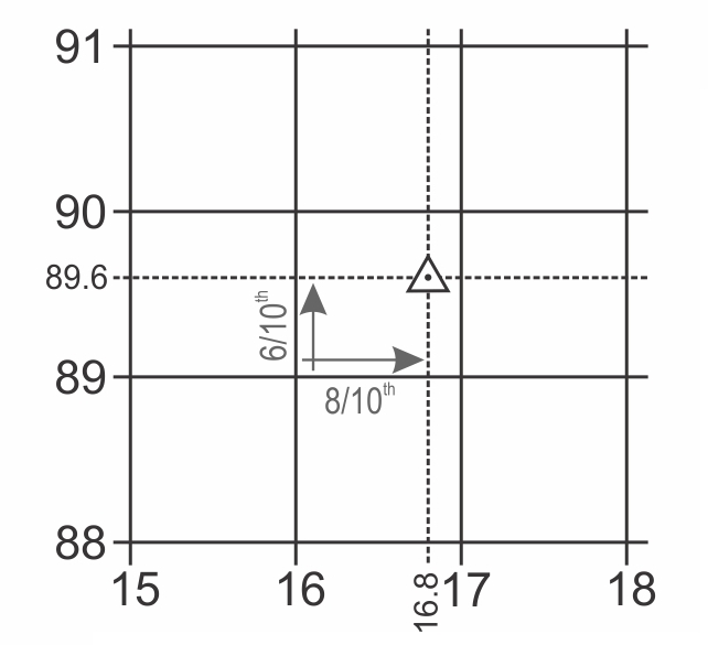
Step 2: Northing. Work bottom-to-top. In the example shown above, the northing is between 89 and 90 – about six-tenths the way up. So, the northing is 89.6 which gets abbreviated to 896.
Step 3: Put it together. The grid reference 168896 (not 896168).
Finally, note that we can derive 6-figure grid references from a full UTM coordinate. Let’s use the gold example one from above: 11U4347825644518. The 11U part is not used in grid references, but we do need the remaining numerical information:
- Easting: the full easting is 434782. Since grid references give estimates to the nearest hundred metres, we want to round off the full easting to the nearest decametre (1 dam = 100 m); in this case, it is 4347.82 dam, which rounds off to 4348 dam. We only want the last three digits, so we end up with a 3-figure easting of 348. If this was on a NTS map, this would be between the blue grid lines of 34 and 35, and much closer to the 35 line.
- Northing: the full northing is 5644518. Following the principles as for the easting, we can think of this as being a value of 56445.18 dam, which rounds off to 56445 dam. We only want the last three digits, so we end up with a 3-figure northing of 445. If this was on a NTS map, this would be halfway between the blue grid lines of 44 and 45.
So, we end up with a grid reference of 348445 (but not 445348).
For an example of determining the 6-figure grid reference of a location when using a NTS map, refer to the Supporting Material.
Map Scales
The world is big. Maps are small. So, real-world sizes have to be reduced in order to fit the landscape onto a map, and the map scale tells us how much size reduction has taken place.
Map scale can be expressed in several different ways:
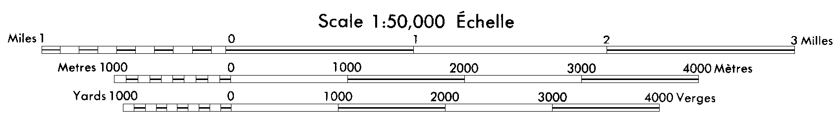
- Graphic scale: a simple line or bar on the map that states the real-world distance (Figure 14.5). It is simple and intuitive to use.
- Ratio scale: one unit of linear distance (e.g., millimetre, inch) on the map represents some number of the same units in the real-world. In the previous section, reference was made to 1:50,000 maps – this simply means that 1 mm on the map represents 50,000 mm in the real-world, or 1 inch represents 50,000 inches, and so on. The standard convention is to use the form 1:n, where n can be any number.
- Verbal scale: typically, a statement that relays the same information as a ratio-type scale. For example: 1 cm represents 1 km is self-explanatory – it means that a distance of 1 cm on the map is equivalent to one kilometre in the real-world (so the ratio scale would be 1:100,000). Slightly more esoteric examples are: 5 cm to 1 km, or 1 cm equals 20 km, neither of which makes complete grammatical or logical sense, but the meaning should be fathomable for any geographer (the ratio scales are 1:20,000 and 1:2,000,000, respectively).
Being able to convert between different types of scale is a useful skill.
We sometimes hear the terms small-scale map, medium-scale map or large-scale map, and it can be confusing. Perhaps the simplest way to think about this is to realize that a large-scale map will show a given feature larger on the map than a small-scale map would. Think about fitting a map of Canada on this page – you have to shrink the country very small in order to do so, and British Columbia would occupy only a small part of the page. This is a small-scale map. Now envisage a map only of British Columbia on this page – obviously, we can make it larger, and so the scale has become larger, although it would still not be considered a large-scale map. An example of a large-scale map is a 1:50,000 map sheet, where the map shows the landscape in fine detail. You may also think of this mathematically: convert the ratio to a fraction, and the smaller the fraction, the smaller the map-scale.
Test your understanding: Which map has the largest scale?
- Map A, 1:40,000
- Map B, 1:4,000,000
Again (because it's important!), map scale always boils down to this basic ratio:
(the length of a feature on the map) : (the real-world length of the same feature)
…and the units must be identical either side.
As an example, on your map the straight-line distance between your house and the shopping mall is 120 mm. In the real-world, this distance is 2.4 km. So, your map’s scale is 120 mm : 2.4 km = 120 mm : 2,400,000 mm = 1:20,000.
Deriving Distances from a Map
Conceptually, this is simple: measure the distance on the map and multiply it by the scale. For example, 45 mm on a 1:50,000 map represents:
45 × 50,000 mm = 2,250,000 mm
in the real-world. Knowing that 1 m = 1000 m, we can convert this distance to 2250 m.
Measuring straight-line distances is easily achieved with a ruler, of course. Alternatively, you could use the edge of a piece of paper and find the map distance and then compare it to the graphic scale bar.
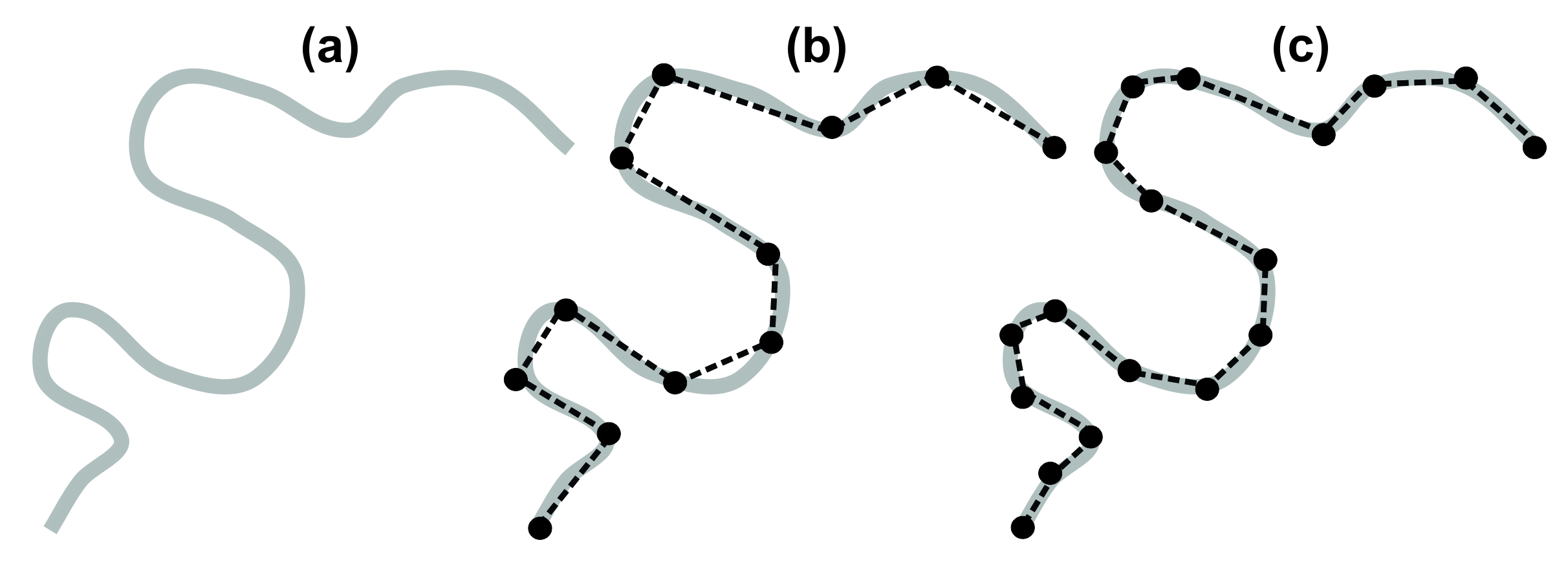
Measuring distances along curvilinear features such as roads and rivers is more complicated. It is possible to use a ruler and then treat the curved lines (Figure 14.6a) as a series of straight segments (Figure 14.6b). Although this method will tend to underestimate the distance, it will certainly give a rough estimate that's usable. Accuracy can be improved by using shorter straight segments (Figure 14.6c), but this comes at a cost of extra time and effort required.
If you are using a hard-copy map, an alternative method of measuring curved lines is to use an opisometer (also called a map measurer).
For instructions on how to derive distances in Google Earth (Web), refer to the Supporting Material.
Finally, there are also trigonometric methods to derive straight-line distances that use geographical or UTM coordinates but these are beyond the purview of this lab.
Deriving Areas from a Map
When calculating the area of objects on a map keep in mind that scales are linear and cannot be applied directly to area calculations. Therefore, although an area 10 cm wide and 20 cm long on a map is 200 cm2 (10 cm × 20 cm = 200 cm2), you cannot take the 200 cm2 and use the map scale to get the area in the real-world. Instead, you must multiply each length by the map scale to get real-world lengths (or lengths on the ground) before multiplying together to get the area.
For example, assume you have a map at a scale of 1:10,000, and you want to work out the area in the real-world for a map area that is 10 cm wide and 20 cm long. Follow these steps:
Step 1: Calculate real-world width: Real-world width = map width × map scale = 10 cm × 10,000 = 100,000 cm = 1 km
Step 2: Calculate real-world length: Real-world length = map length × map scale = 20 cm × 10,000 = 200,000 cm = 2 km
Step 3: Calculate the real-world area: Real-world area = Real-world width × Real-world length = 2 km2
Applying the map scale to the map area directly would give an area of 2,000,000 cm2 = 2,000 m2 = 0.002 km2 which is far too small.
Remember: scales are linear and cannot be applied directly to area calculations.
Useful Unit Conversions for Mapping
Area Conversions
Sometimes it is necessary to convert areas expressed in square kilometres (km2) to other units such as hectares (ha). The easiest way to do this is to convert to square metres (m2).
First up, let us convert 1 km2 to m2 (Figure 14.7a). In other words, we have a square that has a length and width of 1 km.
Step 1: Convert the length and width of each side of the square from km to m. We know that there are 1,000 m in each 1 km, therefore: Length (= width) = 1 km × 1,000 = 1,000 m
Step 2: Calculate the area of the square in m2: Area (m2) = Length(m) × width(m) = 1,000 m × 1,000 m = 1,000,000m2
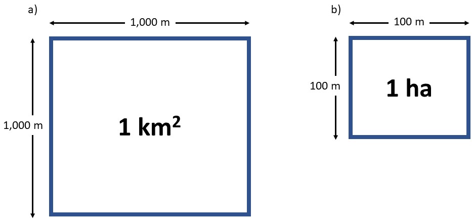
We can convert 1 ha to m2 using the same process (Figure 14.7b). In this case, we have a square that has a length and width of 100 m, and so we can skip Step 1, where we converted the length/width to m. This simplifies to:
Calculate the area of the square in m2: Area (m2) = Length (m) × width (m) = 100 m × 100 m = 10,000m2
In summary,
- 1 km2 = 1,000,000 m2,
- 1 ha = 10,000 m2,
- and hence, [latex]1 km^{2} = \dfrac{1,000,000}{10,000} = 100 ha[/latex].
Degree Conversions
Coordinates stated in degrees, minutes and seconds (DMS) can be converted to decimal degrees (DD), and vice versa, using ratios of
- 60 seconds in a minute,
- 60 minutes in a degree, and
- 3600 seconds in a degree.
For example, coordinates for a location are given in DMS as 49°11’15’’. Convert to DD as follows:
[latex]= 49 + \dfrac{11}{60} + \dfrac{15}{3600}[/latex]
[latex]= 49.1875 ^{\circ}[/latex]
Converting from DD to DMS requires four steps. Coordinates for a location are given in DD as 49.8675°. Use these four steps to convert to DMS:
Step 1: Obtain the degrees from the number in front of the decimal point = 49°
Step 2: To obtain the minutes, multiply the decimal by 60 minutes.
= 0.8675 × 60
= 52.05′
The number of minutes is the number in front of the decimal point (52).
Step 3: To obtain the seconds, multiply the decimal from Step 2 by 60 seconds.
= 0.05 × 60
= 03″
Step 4: Put together the degrees, minutes and seconds obtained from steps 1-3. The coordinates in DMS are 49°52′03″.
Lab Exercises
This lab consists of four exercises in which you will practice
- Deriving geographical coordinates, converting between units and using them to find locations on maps and in Google Earth (Web).
- Deriving UTM coordinates and using them to find locations on maps.
- Working with map scales.
- Calculating distances from maps.
You will need a calculator, plus an internet connection to download a map and access Google Earth (Web). Some of the exercises may be easier if you are able to print Figure 14.1. The exercises should take you 1½ to 3 hours to complete.
EX1: Geographical Coordinates
- Using only Figure 14.1, address the following questions:
- Derive the latitude and longitude of the 669-metre summit about a kilometre NW of McKinley Reservoir. Express your final answer to the nearest 10" (i.e. round off to 00", 10", 20", etc.).
- What feature is at 49° 55' 40" N, 119° 23' 30" W?
- Open Google Earth (Web) and describe what feature is present at 43° 38' 33" N, 79° 23' 13" W.
- You are exploring BC's beautiful landscapes and are wondering if this is a safe place to pitch your tent. Your GPS receiver indicates that you are here: 54.1895° N, 131.6471° W.
- Convert the coordinates to DMS. Show your work.
- Type these coordinates into Google Earth. Where are you?
- Do you want to camp here? Why or why not?
- Download the 1:50,000 NTS map sheet 01N10 (St. John's) 8th edition [PDF]. Use only this map for the following questions:
- Derive the latitude and longitude of the steel mill by Octagon Pond, Paradise (lower-left part of map). Express your final answer to the nearest 10".
- What feature is at 47° 34' 13" N, 52° 40' 55" W? PS: Do you happen to know why this place is famous?
- Convert these coordinates to decimal degrees (DD) correct to 4 decimal places.
EX2: UTM Coordinates
- Using only Figure 14.1, address the following questions:
- Derive the full UTM coordinate of the 669-metre summit a kilometre NW of McKinley Reservoir. Express your final answer to the nearest 50 m (i.e. round off to …00m or …50m; this is equivalent to the nearest whole millimetre of measurement on the original map).
- Convert your answer for (a) to a 6-figure grid reference.
- What do you find at 11 U 328600 5533850?
- If you worked at the feature at 207306, what are you most likely doing?
- Use the 1:50,000 NTS map sheet 01N10 (St. John's) 8th edition [PDF] (same map you used in Q4).
- Derive the full UTM coordinate of the South Head navigation light at the entrance to St. John's Harbour (see the map's legend for the symbol for a navigation light; you will also have to search the map for the UTM zone information). Express your final answer to the nearest 50 m.
- Convert your answer for (a) to a 6-figure grid reference.
- What feature has a UTM coordinate of 22 T 354100 5278750?
- Using either Figure 14.1 or the 1:50,000 NTS map sheet 01N10 (St. John's) 8th edition [PDF], identify a location where you would like to eat lunch.
- Derive the full UTM coordinate for the location.
- Explain why it is a good place to eat lunch and how you know this. Hint: consider the colour, map legend, what you may be able to view from the location...
EX3: Map Scales
- Address all of the following to get some practice using map scales:
- On a 1:50,000 map, what does a length of 50 mm represent?
- On a 1:250,000 map, what does a length of 50 mm represent?
- The straight-line distance from point A to Point B is 14 km. What length would this be on a 1:20,000 map?
- Convert the verbal scale One centimetre equals four kilometres to a ratio scale.
- Assume that you need to use a part of a standard 1:50,000 NTS map in your next term paper, but you had to shrink the map in order to fit it on the page. On your new map, the length of ten grid squares is 137 mm.
- Is your map a smaller scale or larger scale than 1:50,000? Explain.
- Calculate the scale of your map.
EX4: Distance
- Use Figure 14.1 to determine the following distances:
- How long is the runway at Kelowna airport (in metres)?
- What is the straight-line distance (in metres) between the 636-metre summit of Mount Dilworth and the 595-metre summit at 262346?
- What is the shortest distance (in kilometres) by road between the two junctions at 254343 and 286323?
- Open Google Earth (Web).
- Use Google Earth (Web) to check your answers to Question 10. Refer to Google Earth procedures in Supporting Material.
- Explain why your answers calculated in Q10 and measure in Q11a are not identical.
- In previous exercises we assumed that the cutting, pasting and uploading and/or printing of the map section on Figure 14.1 did not change the map scale. It is now time to check this, so that you can calculate the area of Knox Mountain Park accurately. If you have not printed Figure 14.1, you can measure the distances on your screen, just remember that you must not change the magnification of your screen between measurements in this exercise.
- Unfortunately, this map section does not contain the graphic scale. However, you know that the blue UTM grid represents squares that are 1000 m wide and 1000 m tall. Using your ruler, measure the width of one grid square (in mm) and use this distance to calculate the scale of the map as printed/appears on your screen. Express it as a ratio. Show your work.
- Use the map scale calculated in (a) to calculate the area of Knox Mountain Park in m2, km2 and ha. Show your work.
Reflection Questions
- One of the most fundamental issues in geography is location - Where am I? Where is this place? Where is that place in relation to the other place? Think about the different ways in which location can be defined and specified. Explain how you would tell someone exactly where you are right now, the square metre of Earth's surface that you are currently occupying! How would your description be different if you simply wanted to give the general location of the town that you are in?
- You have arranged a hiking trip for yourself and some inexperienced friends. You have printed out some UTM topographic maps and brought along a couple of GPS units (you knew your friends wouldn’t). Unfortunately, none of them know how to read a map or use GPS! How would you describe to your friends how to locate themselves on the map using the UTM coordinates obtained from the GPS unit?
- Google Maps has crashed, but Google Earth (Web) is fine (somehow) and you need to figure out how to get from Kelowna, BC to Fort St John, BC. You know that you can look up both Kelowna and Fort St John and pin them in Google Earth, and that enabling the Roads layer will give you all major roads in BC. How could you figure out the distances of different path options and choose the quickest route?
Supporting Material
Instructions for Using and Accessing Maps
Contents
How to Derive Geographical Coordinates from a 1:50,000 NTS Map
How to Derive UTM Coordinates from a 1:50,000 NTS Map
How to Derive a 6-Figure Grid Reference from a 1:50,000 NTS Map
How to Measure Distance in Google Earth (Web)
How to Download NTS Topographic Maps
How to Derive Geographical Coordinates From a 1:50,000 NTS Map
First, take another look at Figure 14.1. We are going to get the coordinates of Wilson Landing. Wilson Landing is located in the top-left of the map. A schematic of the location of Wilson Landing is shown on Figure 14.8.
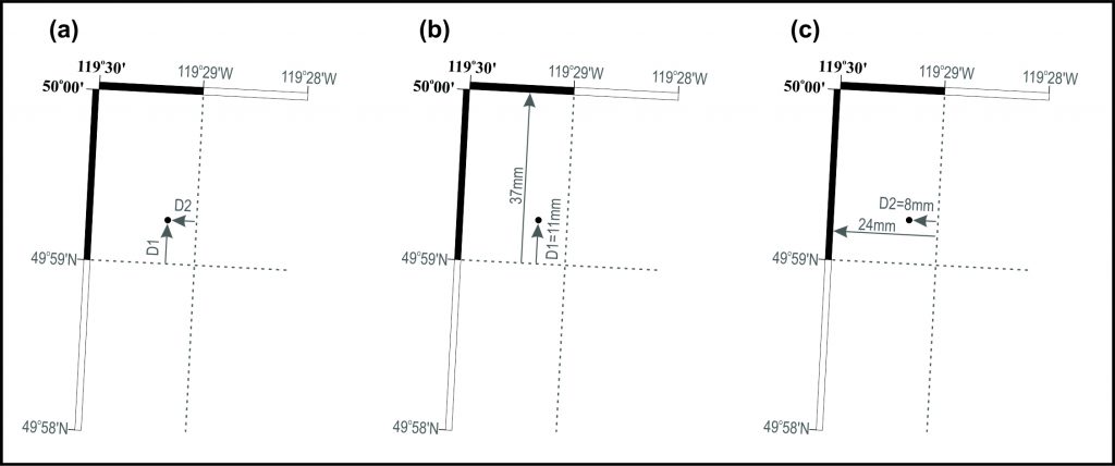
Step 1: Find the approximate location. Using Figure 14.8a, we can estimate the latitude and longitude: the locations is slightly north of 49° 59' N and slightly west of 119° 29' W. Estimating by eye, the arrows indicate that we will add about one-quarter to one-third of one minute of arc to this estimate. To get an answer better than a simple by-eye estimate, we will make measurements on the map. Note that the grey arrows depicting measurements are parallel to the map's neatlines and not the blue grid squares.
Step 2: Derive latitude (Figure 14.8b). We are looking to derive the proportion of one minute of arc that is between the 49° 59' N parallel and Wilson Landing: distance D1. On the original map used in here, the proportion is 11mm:37mm. Therefore, distance D1 must be 11/37th of one minute of arc: [latex]= \dfrac{11}{37} \times 60 \text{ seconds} = 18\text{ seconds}.[/latex]
Step 3: Derive longitude (Figure 14.8c). We are looking to derive the proportion of one minute of arc that is between the 119° 29' N meridian and Wilson Landing: distance D2. On the original map used in here, the proportion is 8mm:24mm. So, distance D2 is 8/24th of one minute of arc [latex]= \dfrac{8}{24} \times 60\text{ seconds}= 20\text{ seconds}.[/latex]
Step 4: Compile. The geographical coordinates of Wilson Landing are 49° 59' 18" N, 119° 29' 20" W.
Back to Supporting Material contents
How to Derive UTM Coordinates From a 1:50,000 NTS Map
Again, we'll use Wilson Landing in Figure 14.1 as our working example.
Step 1: Find the UTM quadrilateral. This information isn't shown on Figure 14.1, but it would be found on the original map sheet; in this case, it happens to be 11U (see Figure 14.9).
Step 2: Derive the Easting. At the top corner of the map sheet we can see the true easting given for one of the blue grid lines: 322000 mE. The grid line to the left is 1000 m away and so must have an easting value of 321000 mE. Wilson Landing lies between the two. To get the best estimate of the easting, we should measure how far it is from the 321000m grid line to our location: in this case, on the original map, it is 13 mm, to the nearest whole millimetre (it's not usually valid to use a finer precision than this). At a scale of 1:50,000, 13 mm represents 650 m in the real-world, and so this distance is added to the 321000m to get our full easting: 321650 mE.
Step 3: Derive the Northing. The top-most horizontal blue grid line has a full northing of 5541000 mN (see the blue number in the upper-left part of Figure 1), and so the next grid line to the south must have a value of 5,540,000 m. Making a measurement on the map, we find that Wilson Landing is about 300 m north of the latter grid line and therefore the full northing is 5540300 mN.
Step 4: Compile. Put it all together to get a UTM coordinate in the format of UTM quadrilateralEastingNorthing: 11U3216505540300.
Back to Supporting Material contents
How to Derive a 6-Figure Grid Reference From a 1:50,000 NTS Map
The 6-figure grid reference, again, for Wilson Landing, is derived from the blue UTM grid and numbers in Figure 14.1.
Step 1: Derive the Easting. Work left to right: Wilson Landing is between grid lines 21 and 22 (interpolated from the blue numbers along the top of map). Moving right from the 21 grid line, Wilson Landing is about six-tenths the distance to the 22 grid line, therefore the easting part of the grid reference is 216 (you can think of it as 21.6, but without the decimal point).
Step 2: Derive the Northing. Working bottom to top, we can see that Wilson Landing is between horizontal grid lines 40 and 41, and about three-tenths the distance between them: so, the northing part of the grid reference is 403.
Step 3: Compile. Put the easting and northing together (EastingNorthing) to get a grid reference of 216403.
Can you see, by inspection, how you can also derive a 6-figure grid reference from the full UTM coordinate?
Back to Supporting Material contents
How to Measure Distance in Google Earth (Web)
To derive a straight-line distance: The bottom icon on the left-hand menu is a ruler. Click this. Mouse-click once to start a line, then double-click at a second point to end the line. Change the units using the dropdown menu adjacent to the distance in the box that pops up in the top right of the screen.
To derive a curved-line distance: The bottom icon on the left-hand menu is a ruler. Click this. Mouse-click once to start a line, single-click at a point to put your second point, single-click at a point to put your third point, and so-on. Double-click at your final point to end the line.
Back to Supporting Material contents
How to Download NTS Topographic Maps
Option 1: If you don't know the map sheet's number: access the Geogratis Topographic Information website and select the Geospatial Product Index - HTML. You can then zoom in or out of the map and the map codes will appear. For example, zoom in on Vancouver: you will first see 92 appear, then a grid with letter codes, and then number-letter-number codes which are the 1:50,000 map IDs; downtown Vancouver is map sheet 92G06. You may get access to the maps directly from here, but if not, record the map sheet number and go to Option 2.
Option 2: If you know the map sheet's number: access Geogratis's ftp site for 1:50,000 map sheets. You will find *.tif and *.pdf files available; these are scanned versions of the original NTS map sheets.
