Lab 09: Surface Water Budget
Gillian Krezoski
Where precipitation goes once it reaches the Earth’s surface can be studied using a water budget, or surface water balance. Similar to a bank account, water can be deposited and stored in the soil profile as soil-water storage. If the soil-water account becomes too full, some of the water flows overland to become surface water. Sometimes additional expenses like environmental use through evapotranspiration can remove some of the water from the bank, and in some locations where usage is high, could create a deficit. This lab will use a simple bucket model to examine soil surface water budgets.
Learning Objectives
After completion of this lab, you will be able to
- Calculate a simple soil surface water budget.
- Understand how water is distributed and utilized at the Earth’s surface.
- Learn about online sources for climate data (Environment and Climate Change Canada).
- Learn about local evapotranspiration resources for agriculture (Farmwest.com).
- Begin to hypothesize how water resources could be impacted by the changing climate.
Pre-Readings
The Water Cycle
The water cycle is the global circulation of water from oceans through the atmosphere back to the oceans or to the land and from there to the oceans by overland and subsurface routes. Water is always on the move. Key aspects of the water cycle are:
- Evaporation, in which water transforms to a vapour, and moves into the atmosphere. It takes place from all surfaces that contain moisture, ranging from a free water surface on the ocean to the moisture on a leaf.
- Precipitation, in which atmospheric water vapour condenses to a liquid or solid form. It falls in various forms – snow, rain, hail, and is also deposited on the surface of the earth by the formation of dew and frost.
- Storage. Water is stored for varying lengths of time in a number of forms and locations including atmospheric moisture, water in swamps and lakes, soil moisture, groundwater, ice in glaciers, and snow on the ground.
- Movement. Water is transferred from one location to another by surface runoff, infiltration from the surface, groundwater flow, and via atmospheric vapour carried by winds.
The most important aspect of the hydrological cycle is not the quantity of water residing in the world’s water bodies and atmosphere at any particular instant but rather the rates at which water is transported from one part of the cycle to another. As it moves, water is constantly reacting with its physical, chemical, and biological environment, changing its state, (liquid, vapour, and solid) and reshaping the face of the earth and allowing life as we know it (Environment and Climate Change Canada: The hydrologic cycle).
Water Budgets
Most physical geography introductory textbooks have a segment discussing water budgets. For example, Christopherson et al. (2019) includes a section called Water Budgets and Resource Analysis. Simply put, water budgets are one method used to account for the gain and loss of water from a defined reservoir. Here we investigate the simple bucket methodology for a water budget, which forms the conceptual basis of many more complicated models of water movement.
The Bucket Methodology
The monthly water bucket methodology was first used in the 1940s and 1950s to improve our understanding of the relationship between climate and agriculture (e.g. to determine irrigation needs). It has been applied in many different ways over the years and although modern models have many more features, a simple bucket model still forms the core of many climate modelling concepts (Figure 9.1).
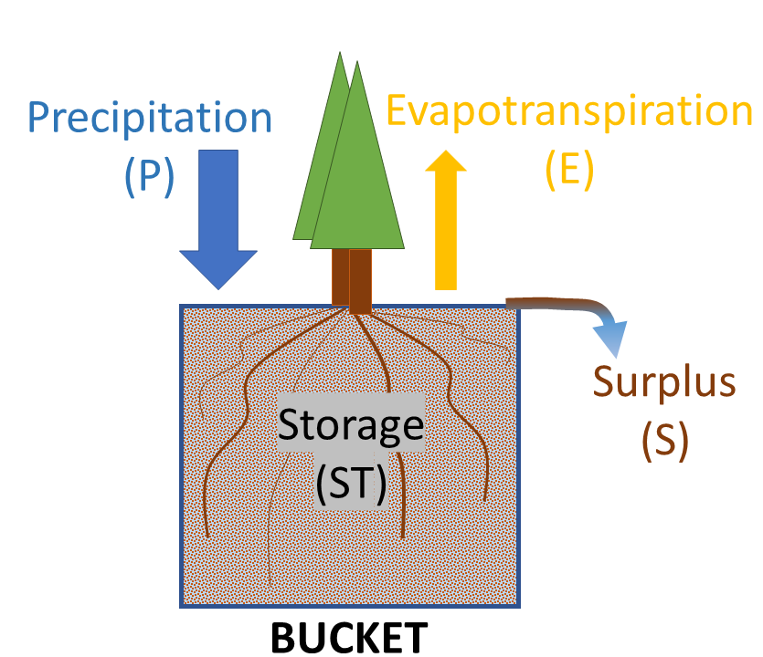
The bucket methodology works as follows:
- Imagine a point on the ground surface of Earth as a bucket (Figure 9.1). As it rains (precipitation, P), water soaks into the soil becoming soil-water storage (ST). This soil-water begins to fill the bucket.
- Water leaves the bucket by evapotranspiration, the name we give to the amount of water that is evaporated (turned from liquid to vapour) or transpired (drawn up by plants and evaporated from their leaves) from all elements of the environment (plants, animals, soil, etc.). This is called utilization.
- If there is more precipitation than evapotranspiration, the bucket will fill. Once there is no more room for water in the bucket (i.e. the bucket is full), the bucket overflows and any more precipitation becomes surplus (S). This water will run off to streams and flow out of the area.
- We can further classify evapotranspiration into two types:
-
- Actual evapotranspiration (AE) – the actual amount of water that is evapotranspired; and
- Potential evapotranspiration (PE) – the amount of water that could be evapotranspired at the current climate conditions if there was ample water available in the bucket.
For example, let us consider a dry, hot and windy desert. In this type of location the potential for evapotranspiration is quite high, because low atmospheric moisture, high air temperature, and wind all increase the rate of evapotranspiration. However, when there is very little water available in the soil or from precipitation, such as in this desert, the actual evapotranspiration is quite low.
Another example is a refrigerator. Potential is related to how hungry you are, but actual is related to how much food you have available in the refrigerator to eat.
- The starting point for a water budget is therefore to compare the inputs (P) to the potential demand (PE). If there is lots of precipitation, or lots of water in storage, then the actual evaporation (AE) might be able to keep up to the potential evaporation.
However, if the precipitation is low, or the soil-water storage is low, then there may not be enough water available for the plants to use and AE might be lower than PE. This can create a water deficit (D) in the environment, where the environment does not have enough water coming in, or contained in storage, to keep up with demand.
Once there is a deficit, plants and the environment are not able to satisfy all of the demands they have for water, which will create stress. A moisture deficit can be a major limiting factor to most biomes (i.e. plant and animal survival).
- The deficit has to be made up with precipitation before the bucket begins to fill up again (soil-water recharge).
Example Bucket Water Budget
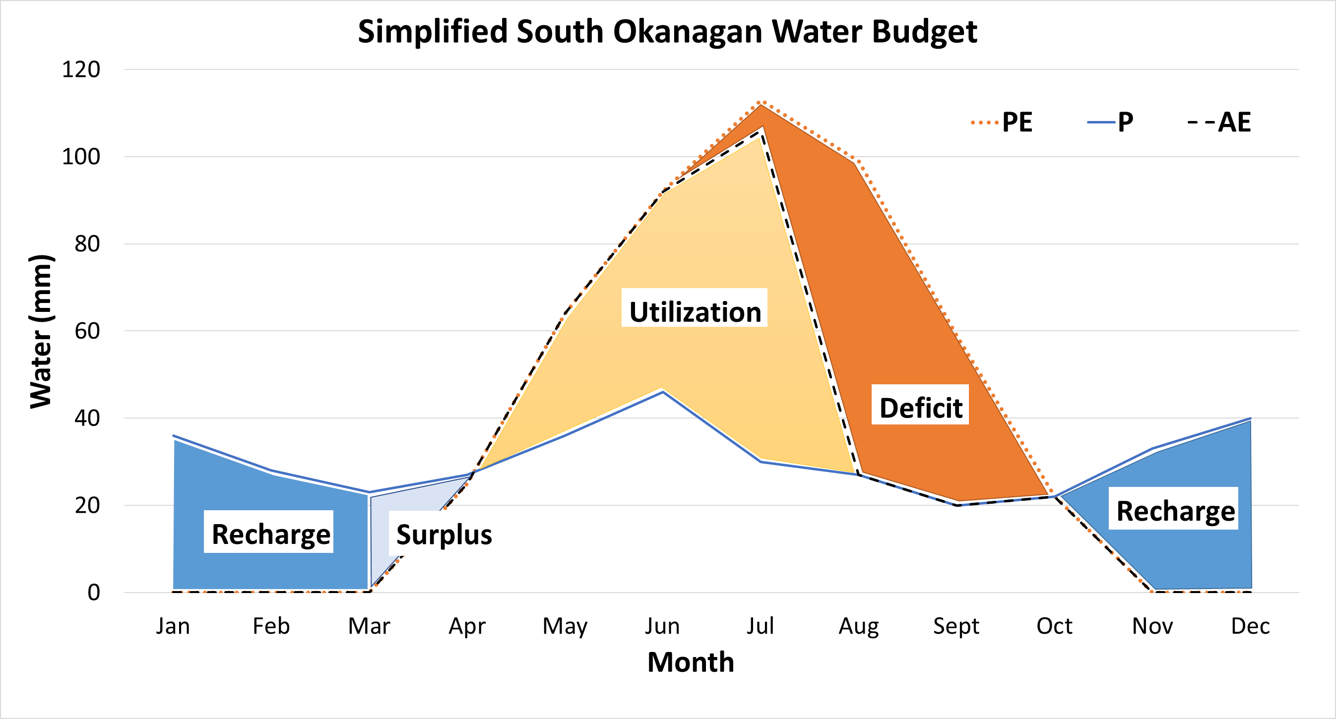
A simplified sample annual water budget of the South Okanagan at elevation (between Penticton and Osoyoos) is included below (Figure 9.2, based on Table 9.1). In this case, the amounts of precipitation, evapotranspiration, surplus and storage are all expressed in millimetres (mm). The size of the bucket, which represents the Water Holding Capacity (WHC) of the soil, has been set to be 150 mm of storage available in the soil column.
| Month | Temp (°C) | PE | P | P – PE (DIFF) | ST | ΔST | AE | D | S |
|---|---|---|---|---|---|---|---|---|---|
| Jan | −10.4 | 0 | 36 | 36 | 109 | 36 | 0 | 0 | 0 |
| Feb | −6.5 | 0 | 28 | 28 | 137 | 28 | 0 | 0 | 0 |
| Mar | −2.2 | 0 | 23 | 23 | 150 | 13 | 0 | 0 | 10* |
| Apr | 2.7 | 25 | 27 | 2 | 150 | 0 | 25 | 0 | 2* |
| May | 7.3 | 64 | 36 | −28 | 122 | −28 | 64 | 0 | 0 |
| Jun | 11.1 | 92 | 46 | −46 | 76 | −46 | 92 | 0 | 0 |
| Jul | 14.3 | 113 | 30 | −83 | 0 | −76 | 106 | 7 | 0 |
| Aug | 13.7 | 99 | 27 | −72 | 0 | 0 | 27 | 72 | 0 |
| Sept | 9.0 | 59 | 20 | −39 | 0 | 0 | 20 | 39 | 0 |
| Oct | 3.0 | 22 | 22 | 0 | 0 | 0 | 22 | 0 | 0 |
| Nov | −4.3 | 0 | 33 | 33 | 33 | 33 | 0 | 0 | 0 |
| Dec | −8.6 | 0 | 40 | 40 | 73 | 40 | 0 | 0 | 0 |
| Total | – | 474 | 368 | – | – | – | 356 | 118 | 12 |
In the winter months precipitation (P) includes some rainfall but mostly snowfall. During this period, the bucket is filling up during a recharge phase, which is expressed in Table 9.1 as storage (ST). Surplus (S) water escapes via stream systems rapidly in the late spring, often causing flooding.
One should note that because of snowmelt occurring in the late spring, the South Okanagan – especially at elevation – is a bit more complex than Table 9.1 suggests. Since that snow already fell as precipitation earlier in the year, it is not accounted for in this simple soil-water balance exercise. In reality, the surplus in the spring is much higher due to the snowmelt.
The South Okanagan is a high-latitude desert so evapotranspiration needs (PE) are quite high during summer. As the summer gets warmer, the soil-water storage (ST) is gradually depleted, actual evapotranspiration (AE) decreases, and a deficit (D) is created.
Vegetation native to the area experiences a deficit all summer and has strategies to survive the low water conditions until some rain appears in the fall. However, agriculture is common in the South Okanagan, with fruit trees and grape vines common crops. These plants are not adapted to the naturally dry environment and would be permanently harmed by the natural summer water deficits. Therefore, farmers supply the plants with extra water through irrigation from reservoirs. This supplementary water is used to fulfill agricultural needs and prevent soil-water deficits that could harm the crops until the winter recharge can occur.
To summarize, evaporation indicates movement of water away from a wet surface into a dry atmosphere. Transpiration is where plants release water from their leaves into the atmosphere that has made it through their root/trunk/branch system. On a hot day, trees transpire more than cold days (tree sweat!). Once the growing season starts (typically after freezing temperatures cease), plant needs in the environment increase and evapotranspiration increases. Growing seasons can vary throughout the province based on temperatures and precipitation. If the summer months experience dry periods, and plants begin using water from the soil-water storage (the bucket), eventually the soil-water storage might empty, and irrigation will be needed to reduce the local water deficit.
Lab Exercises
In this lab you will:
- Look at Environment and Climate Change Canada Climate Normals data (30-year datasets) to understand average local annual ‘inputs’ into your given station.
- Examine local evapotranspiration (an output from your water budget) using Farmwest.com, an agricultural resource used by farmers to plan for irrigation needs in times of deficits.
- Complete a modeled water budget local to your (or your school’s) area to determine where your water goes once it reaches the Earth’s surface:
- Into the bucket as soil-water storage
- Out of the bucket as surplus (to become surface water flows)
- Out of the bucket via evapotranspiration (environmental utilization)
- Create your own water budget graph similar to Figure 9.2.
EX1: Reviewing Climate Normals
Step 1: Visit the Environment and Climate Change Canada Canadian Climate Normals webpage (1981-2010 data).
Step 2: Your instructor will assign you a station name local to the area you are studying. Navigate to the station name.
Station Name:
Step 3: Scroll down to see a climograph where average monthly temperatures (lines) and average monthly precipitation (bars) are plotted together over the course of a year using Climate Normal data (30-year data-set from 1981-2010).
Step 4: Take a screen capture of the climograph for use with the Reflection Questions at the end of this lab.
Step 5: Click on the View Data Table tab in the lower middle portion of your screen below the Temperature and Precipitation graph. The data that are used to plot the climograph are included here. You might want to refer to this data in your answers if you cannot determine numbers from the climograph on your screen. If so, click on Download Data in the bottom right of the new screen.
Once you have completed Step 1 through Step 5, answer the following questions:
- Briefly describe quarterly (Jan-Mar, Apr-Jun, Jul-Sept, Oct-Dec) precipitation patterns at your study location. Be sure to identify the
- predominant precipitation forms, i.e., snow or rain.
- driest month.
- wettest month.
- Briefly describe quarterly (Jan-Mar, Apr-Jun, Jul-Sept, Oct-Dec) temperature patterns at your study location. Be sure to identify the
- hottest month.
- coolest month.
- the approximate month(s) during which temperatures start warming enough to melt snow.
EX2: Examining Evapotranspiration
Now that we are familiar with seasonal precipitation and temperature patterns in your study area, we will examine environmental evapotranspiration needs. Farmers often use a website called Farmwest.com to view local precipitation inputs, and view evapotranspiration (ET) outputs so they know how much to water their plants in order to keep water in soil-water storage for their crops to use.
The site calculates the potential evapotranspiration assuming there is always sufficient soil moisture in storage, so that irrigators can determine how much water they need to add to the soil each day to keep the soil moisture storage topped up. Farmwest calculates evapotranspiration for a standard grass crop (like a typical garden lawn). Farmers can calculate ET for their particular crop based on standard calculations and may have to use more or less water than a typical grass lawn. How, when, and for how long, farmers irrigate is a complex science.
Step 1: Navigate to the Evapotranspiration page on the Farmwest website.
Step 2: On the website, enter the station information provided by your instructor for your study location. For Select Date Range use January 1 – December 31 of the previous full year. Click GO. Note that we are using a different date range than our Climate Normals (1981-2010) because 1991-2020 Climate Normals data are not available yet. This is because not all current station data is available for 2010 or earlier on Farmwest.com.
Station information:
Province:
Region:
Station:
Step 3: Scroll down to the two graphs at the bottom of the screen. The upper graph shows evapotranspiration (ET). The green curve is the historical average, and yellow line is the current year. The lower graph shows precipitation events throughout the year.
The graph of evapotranspiration over the year can be presented in two ways. By default it plotted as a cumulative graph on the Farmwest website, where the total ET over the season can be seen. This graph will rise steadily from zero at the start of the graph and will be steepest when daily ET is highest. This type of plot is useful for tracking the total amount of water needed for irrigation over a whole season.
Step 4: Go back to the top of the page where you entered your settings and find the small tick box where you can also choose Not cumulative in graphical display. Click on this option, then click GO again, and re-examine the graph. Now, the daily amount of ET is shown. This graph will rise and fall over the year as climate conditions change and is useful for seeing how daily climate impacts ET. It may be helpful to download the data by clicking the dropdown menu for each graph and selecting Download CSV.
Once you have examined the graphs, answer the following questions. Limit your answers to 1-2 sentences.
- A plot of daily evapotranspiration over one year is a curve with the highest point in the summer and lowest in the winter. Explain why based on your understanding of evaporation and transpiration.
- Examine the local precipitation events and the yellow line indicating evapotranspiration. Is there a relationship between these two variables? Why or why not?
- What other data set would give you some information about the changes to evapotranspiration over time? Why?
- Precipitation events occur in the winter, but the evapotranspiration curve does not change. Why is this?
A water budget can be useful for city planning and for irrigations needs. Indeed, after examining water budgets, city planners and engineers in the Okanagan built reservoirs to capture spring runoff for agricultural and city needs.
In this exercise you will complete a water budget local to your area.
Water Budget Location:
- Complete water budget for your location using the Water Budget Worksheet provided in Worksheets. Your instructor will provide you with the WHC for your location, and the first three columns of data (Temp, PE and AE). Instructions on how to complete the budget are provided in the Supporting Material. You instructor may also provide additional instructions.
Once complete, answer the following questions in 2-3 sentences. Remember, this is individual work.
- What is the driest month (lowest Precipitation), and what is the month of greatest moisture stress (highest Deficit)? Are they the same? Explain your answer.
- What is the wettest month (highest Precipitation), and what is the month of greatest moisture surplus (highest Surplus)? Are they the same? Explain your answer.
- What is causing most of the seasonality: annual temperature differences or precipitation? Explain your answer. Be sure to consider Potential Evapotranspiration (PE) in your discussion.
EX4: Plotting a Water Budget
- Plot your water budget data using Excel (or similar software) to create a visual water budget. Refer to Figure 9.2 as an example.
- Plot your PE, P and AE values for the year.
- Draw by hand (and scan back in) or use PowerPoint or Word to create polygons for Recharge, Deficit, Utilization and Surplus zones. Note that recharge ends once the WHC has been reached.
- Be sure to include a descriptive title, axis labels with units, and an appropriate legend.
Reflection Questions
In general, it is accepted that British Columbia’s climate will become hotter and drier in most places due to climate change. Considering precipitation, temperature, and evapotranspiration (both AE and PE) examined in this lab, take 15-20 minutes to answer the following questions:
- How do you think climate change might impact your study area’s water budget in 50 years? Include trends in inputs (P) and outputs (PE, AE) in your discussion and explain why. Be sure to mention deficits and surpluses as well.
- What sorts of things can be done to remediate future water budget challenges? Include at least three examples in your discussion. If you mention a reservoir or similar, refer to your water budget and explain where the water would come from. Can human usage be changed, given that populations are likely to increase?
- Describe how your Farmwest.com evapotranspiration curve will change as the climate changes. How would this influence farmers’ actions for their crops?
- The simple monthly bucket model used in this lab considered the soil-water storage as a bucket. Is this strictly true of the ground? Describe where else water in the soil goes, and when during the year this is most likely to occur. Review the water cycle if necessary.
Worksheets
Water Budget Worksheet
- Lab 09 Water Budget Worksheet [Word]
- Lab 09 Water Budget Worksheet [ODT]
- Lab 09 Water Budget Worksheet [PDF]
Supporting Material
How To Do A Water Budget Analysis
- Your instructor will supply mean monthly temperature, PE and P, plus a value for the water holding capacity (WHC) for the soil at your site. The WHC is equal to the maximum value of soil water storage (ST).
- You can start your calculations at any time in the water balance, preferably at a time you know something about the soil moisture conditions (i.e. either full or empty), e.g., assume soil moisture is full – at WHC – in January: enter your WHC value in the ST column for January.
- Calculate P − PE (DIFF) for your location.
- Determine your change in storage (ΔST) value based on the DIFF value
If the DIFF is positive, there is extra water, so
-
- Fill up the soil moisture reservoir (if applicable) if it is not full (equal to the WHC). ΔST will be positive.
If ST (prior month) + DIFF is greater than WHC,
ΔST = WHC − ST (prior month)
Remainder of DIFF becomes S (see step 8, below).
If the DIFF is negative, there is a water need
-
- Determine the amount of moisture to be extracted from the soil. ΔST will be negative.
If ST (prior month) + DIFF is greater than zero, then there is sufficient soil water remaining
ΔST = − DIFF
If ST (prior month) + DIFF is less than 0, the soil moisture storage is empty,
ΔST = − ST (prior month), or 0
Remainder of DIFF becomes D (see step 7, below)
- Calculate ST
If DIFF is negative
ST (current month) = ST (prior month) + ΔST (current month)
If DIFF is positive
If ST previous month = WHC
ST (current month) = WHC
If ST previous month is less than WHC
ST (current month) = ST (prior month) + DIFF
OR
ST = WHC if (ST previous month + DIFF) is greater than WHC
- Calculate AE
If DIFF is positive (more than enough water from precipitation for the month)
AE = PE
If DIFF is negative (we are taking water out of the bucket, or ST)
AE = P − ΔST
D = PE − AE
If DIFF is negative
S = 0
If DIFF is positive then
If ST (prior month) = WHC
S = DIFF
If ST (prior month) is less than WHC
S = DIFF − (WHC − ST prior month)
- Balancing the budget
Continue your calculations for all months of the year until you fill in the table and return to the month you started with. If at this point your ST is not the same as the value you began with, you need to repeat the entire procedure until you balance the water budget, and the values for ST in the starting month match. Very rarely you may have to repeat the entire procedure twice to balance the water budget.
- Check your results using this annual balance: Annual AE + Annual D = Annual PE and Annual AE + Annual S = Annual P
References
Christopherson, R.W. et al., (2019). Geosystems: An Introduction to physical geography (4th ed). Pearson Canada Inc.
Environment and Climate Change Canada. (n.d.). The hydrologic cycle. Government of Canada. https://open.canada.ca/data/en/dataset/1b9ef470-5575-5986-a3e6-c18f49402e99.
Environment and Climate Change Canada, (n.d.). Canadian climate normals 1981-2010 station data. Government of Canada. https://climate.weather.gc.ca/climate_normals/index_e.html.
Farmwest.com (2020). Evapotranspiration. https://farmwest.com/climate/calculators/evapotranspiration/.
Web WIMP version 1.02. (2009). Implemented by K. Matsuura, C. Willmott and D. Legates at the University of Delaware in 2003.
