Chapter 9: Analysis Of Survey Data
9.2 Identifying Patterns
Data analysis is about identifying, describing, and explaining patterns. Univariate analysis is the most basic form of analysis that quantitative researchers conduct. In this form, researchers describe patterns across just one variable. Univariate analysis includes frequency distributions and measures of central tendency. A frequency distribution is a way of summarizing the distribution of responses on a single survey question. Table 9.2 presents the frequency distribution for just one variable from the Saylor Academy (2012) older worker survey. Table 8.2 presents an analysis of the item mentioned first in the codebook excerpt given earlier, on respondents’ self-reported financial security.
| In general, how financially secure would you say you are? | Value | Frequency | Percentage |
| Not at all secure | 1 | 46 | 25.6 |
| Between not at all and moderately secure | 2 | 43 | 23.9 |
| Moderately secure | 3 | 76 | 42.2 |
| Between moderately and very secure | 4 | 11 | 6.1 |
| Very secure | 5 | 4 | 2.2 |
As you can see in the frequency distribution on self-reported financial security, more respondents reported feeling “moderately secure” than any other response category. We also learn from this single frequency distribution that fewer than 10% of respondents reported being in one of the two most secure categories.
Another form of univariate analysis that survey researchers can conduct on single variables is measures of central tendency. Measures of central tendency tell us what the most common, or average, response is on a question. Measures of central tendency can be taken for any level variable for ordinal-level variables. Finally, the measure of central tendency used for interval- and ratio-level variables is the mean. To obtain a mean, one must add the value of all responses on a given variable and then divide that number of the total number of responses.
In the previous example of older workers’ self-reported levels of financial security, the appropriate measure of central tendency would be the median, as this is an ordinal-level variable. If we were to list all responses to the financial security question in order from lowest dollar value to highest dollar value, the middle point in that list is the median. For these purposes, we will pretend that there were only 10 responses to this question. Table9.3, Distribution of responses and median value on workers’ financial security”, the value of response to the financial security question is noted, and the middle point within that range of responses is highlighted. To find the middle point, we simply divide the number of valid cases by two. The number of valid cases, 10, divided by 2 is 5, so we are looking for the 5th value on our distribution to discover the median. As you will see in Figure9.3, Distribution of responses and median value on workers’ financial security”, that median value is $128,000.
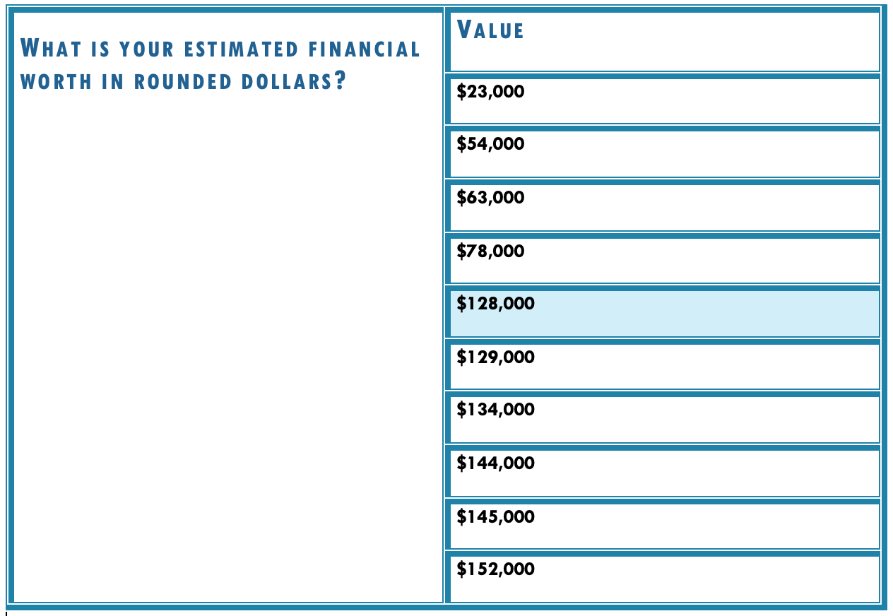
Figure 9.3 Distribution of responses and median value of workers’ financial security
We can learn a lot about our respondents simply by conducting univariate analysis of measures on our survey. We can learn even more, of course, when we begin to examine relationships among variables. Either we can analyze the relationships between two variables, called bivariate analysis, or we can examine relationships among more than two variables. This latter type of analysis is known as multivariate analysis.
Bivariate analysis allows us to assess co-variation among two variables. This means we can find out whether changes in one variable occur together with changes in another. If two variables do not co-vary, they are said to have independence. This means simply that there is no relationship between the two variables in question. To learn whether a relationship exists between two variables, a researcher may cross-tabulate the two variables and present their relationship in a contingency table. A contingency table shows how variation on one variable may be contingent on variation on the other. Let’s take a look at a contingency table. In Table 9.4 “Financial security among men and women workers age 62 and up”, two questions have been cross-tabulated from the older worker survey: respondents’ reported gender and their self-rated financial security.
| Self-rated financial security | Men | Women |
| Not financially secure (%) | 44.1 | 51.8 |
| Moderately financially secure (%) | 48.9 | 39.2 |
| Financially secure (%) | 7.0 | 9.0 |
| Total | N=43 | N=135 |
You will see that a couple of the financial security response categories have been collapsed from five in Table 9.2 to three in Table 9.4. Researchers sometimes collapse response categories on items such as this in order to make it easier to read results in a table. You will also see that the variable “gender” was placed in columns and “financial security” is displayed in rows. Typically, values that are contingent on other values are placed in rows (a.k.a. dependent variables), while independent variables are placed in columns. This makes it pretty simple to compare independent variable across categories. Reading across the top row of our table, we can see that around 44% of men in the sample reported that they are not financially secure while almost 52% of women reported the same. In other words, more women than men reported that they are not financially secure. You will also see in the table that the total number of respondents for each category of the independent variable is in the table’s bottom row. This is also standard practice in a bivariate table, as is including a table heading describing what is presented in the table.
Researchers interested in simultaneously analyzing relationships among more than two variables conduct multivariate analysis. If we hypothesized that financial security declines for women as they age but increases for men as they age, we might consider adding age to the preceding analysis. To do so would require multivariate, rather than bivariate, analysis. We will not go into detail here about how to conduct multivariate analysis of quantitative survey items, but we will return to multivariate analysis in Chapter 16 “Reading and Understanding Social Research”. In Chapter 16 we will discuss strategies for reading and understanding tables that present multivariate statistics.
