11. Beyond Hypothesis Testing

In this chapter we will introduce some big concepts that go beyond hypothesis testing. The three big concepts we need to cover to finish off our coverage of inferential statistics are effect size, power and confidence intervals. Effect size measures just how big a difference between means is, or just how much variability a regression model explains. Effect size is a vital piece of any inferential statistics to complement tests of statistical significance. Power is a critical concept whenever we test a statistical hypothesis – the power to find statistical significance if the research hypothesis is in fact true. And confidence intervals are another approach to inferential statistics that offers an alternative to hypothesis testing. All three of these concepts are extremely important, and they only got left until the end so that we could get all the way through our tour of the full range of statistical tests and techniques first, before zooming out again to these big, important ideas that complement hypothesis testing procedures.

When a hypothesis test reveals that there is a significant difference between means, the question remains… how big was the difference?

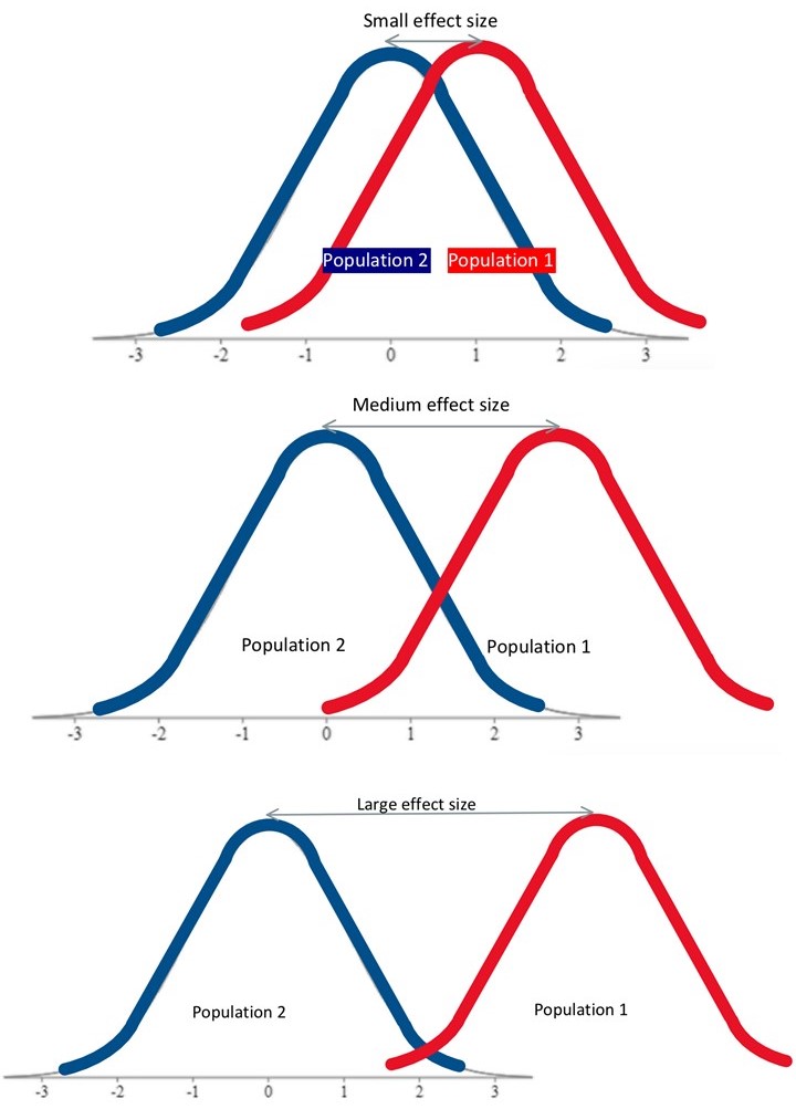
Measures of effect size seek to quantify just how big the effect was of an experiment. For each test of statistical significance, there is a corresponding test of effect size. We already looked at r-squared as the measure of effect size for a correlation, but we have not yet discussed effect size measures for differences between means. Effect size metrics increase with greater differences between the means we are comparing. But how much of a distance between two means is a good, or large effect size and how much is not so good, or small effect size?

Cohen’s d is the most popular measure of effect size, and it is very easy to use. To calculate Cohen’s d, we just take the difference between two means and divide by the standard deviation for the distribution of individuals. The formula shown here is to find the effects size of the difference between means in a situation in which we know the comparison population standard deviation, so the same scenario in which we would conduct a single-sample Z-test to determine whether the difference between means is statistically significant.

Of course, we do not know μ₁, the research population mean, so we must use the sample mean M as the estimate in its place.

Once we calculate Cohen’s d, we can place it on this relative scale to judge the effect size. A Cohen’s d of 0.2 is small, 0.5 is medium, and 0.8 is considered large. 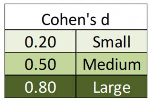So if our two means are a whole standard deviation apart, then we have a very good effect size. Together with a finding of statistical significance from a Z-test, we would have excellent evidence to suggest there is a true difference between the means we were comparing. If, on the other hand, we have a significant Z-test results, but a small effect size, then the difference between the means might be statistically significant, but perhaps it is not such an important difference. This is a common pattern when a research study has a very large sample size, such that it is “over-powered.” The concept of power will come up a little later in the chapter.

Such a situation came up when researchers conducted effect size analyses on the many clinical trials published to establish the efficacy of antidepressant drugs like SSRIs on the symptoms of depression. Once they looked at effect size, they realized that although antidepressants had a statistically significant effect on symptoms, it was a fairly small effect. This called into question the true clinical efficacy of these medications, the most widely prescribed class of psychotropic medication on the planet. Now scientific journals are far more cautious and require researchers to report not just tests of statistical significance, but also tests of effect size, to help the reader interpret the results.

The next concept on our bucket list is power. Statistical power is defined as the probability that the study will produce a statistically significant result if the research hypothesis is true. In other words, when there is a true difference between means, will we be able to detect that? Or will we miss that fact and make a Type II error, failing to reject the null hypothesis when it is false? Power is important, and it directly depends on two factors we have already focused on. Effect size, or the difference between means, is one factor that impacts power. The other factor is sample size, which translates into the width of the distributions being compared.  As you will see, power has to do with minimizing the amount of overlap between distributions, which can be minimized with a) a robust difference between means and b) narrow distributions.

Recall that in hypothesis testing comparing two means, we use the distribution of sample means as the comparison distribution. The standard deviation (i.e. the width of the distribution) is found by dividing by the square root of sample size.

Thus, as sample size increases, the distribution becomes narrower.

Some illustrations will help you picture how these two elements play into power. First, let us examine the relationship between effect size and power, in a simple situation of comparing the means of two distributions.

In these images, the shading under the population 1 distribution represents power. Where does the shading start? Where the cutoff sample score falls on the population 2 distribution. 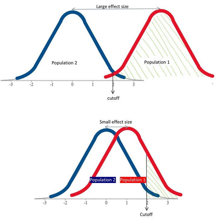The cutoff score for a Z-test that is two-tailed, with .05 significance level, would be at +/- 1.96. Here the shading starts at about Z=2 on the population 2 curve, and continues to the end of the population 1 curve. As you can see here, if the distance between distributions is robust, so the effect size is large, then we have good power. We will have a pretty good chance of detecting a true significant difference. We might think of this as having enough “good variance”. On the other hand, if we have a very modest distance between distributions, so the effect size is small, then the distributions overlap too much, leaving little shaded area. In this scenario, then, we have little chance of rejecting the null hypothesis even when we should.

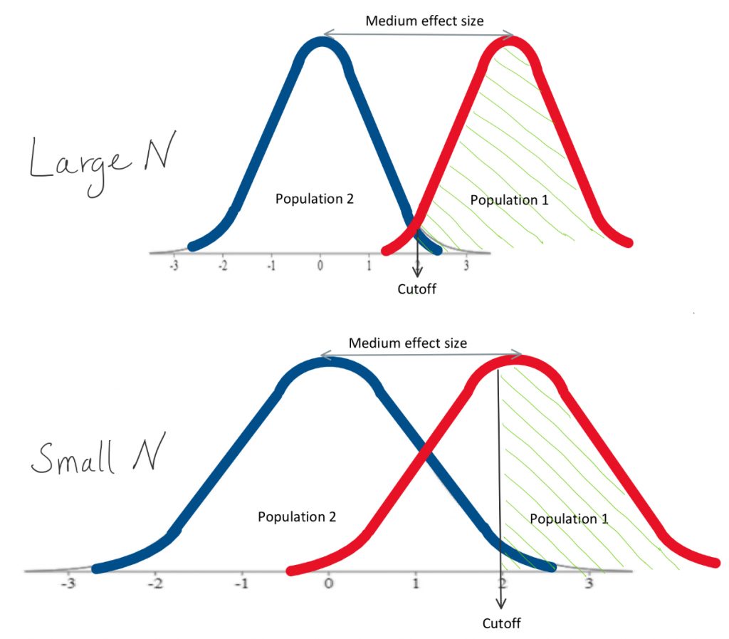The other factor that determines statistical power is sample size, which plays into the width of sampling distributions. When we have a large sample size, the distributions are narrower, and thus there will be less overlap between them. With effect size held constant, just widening the distributions is enough to bring us from very good power to rather poor power. We can think of this as having too much “bad variance”.

So of course, to maximize power we would like to have a large effect size and a large sample size. In reality, of course, we have little control over effect size. As an example, either our insomnia medication helps people sleep a lot longer, or it only helps them sleep a little longer. There is little we can do about just how much of an impact our medication has over sleep. What we researchers can do, though, is make sure that our statistical analysis is based on data from many participants. Even with a moderate effect size, if we have a large sample, we will have nice narrow distributions and thus have a very good shot at detecting a statistically significant result if our medication does help people sleep… even if it is only a modest boost.

Let us take a look at how we can calculate power precisely for the simplest research design we have encountered – a Z-test.

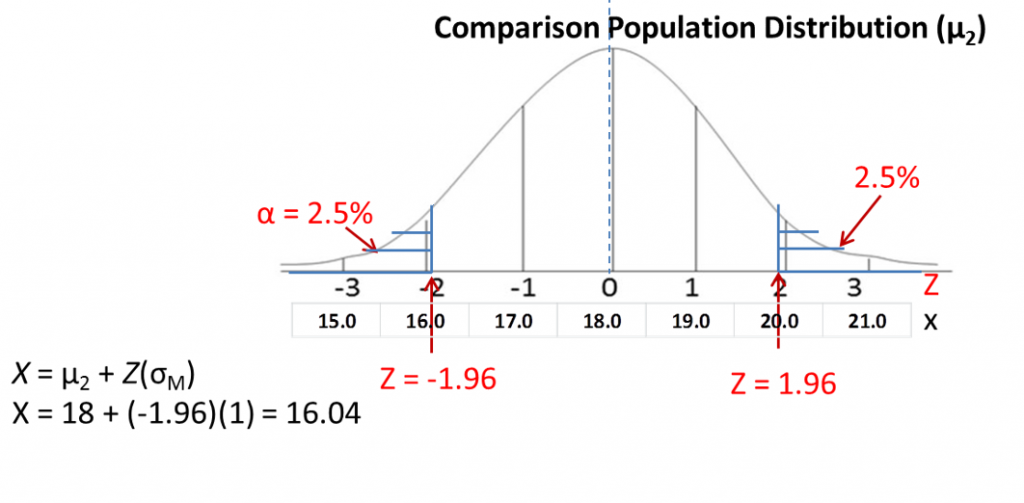First, we draw out the comparison population distribution using the mean and standard deviation we identified from Step 2 of hypothesis testing. On a sketch of the normal distribution, map Z-scores to raw scores (X). In this example, the mean of the comparison distribution is 18, with a standard deviation of 1. As you can see, as Z-scores go up by one, so does the raw score. And as the Z-scores go down by one, so does the raw score.

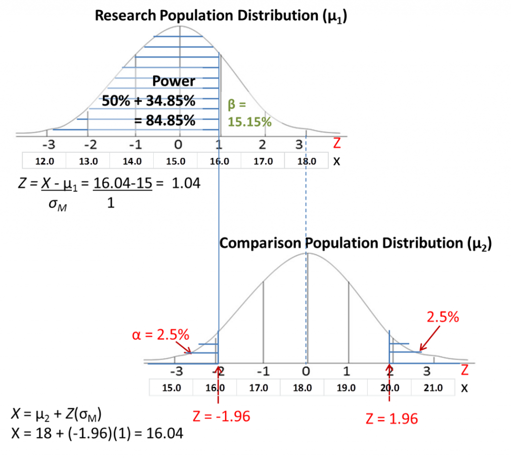
Next, we draw out the research population distribution using the research sample mean M that we calculated for step 4 of hypothesis testing as centre and σ_M as standard deviation. Align the distributions according to the raw scores. Here the sample mean is 15, so we line it up the centre of this new distribution with a raw score of 15 on the comparison distribution.

Next, draw a line straight up from your cutoff score. Shade in everything from there toward the side of the distribution that is away from the middle of the comparison distribution.

Either visually estimate the Z-score where the shading starts on the research population distribution, or find the precise Z-score mathematically by converting the Z-score cutoff to a raw score on comparison distribution, then converting that raw score to a Z-score on the research population distribution. I have shown you what those conversions would look like in the illustrations.

Finally, find the shaded area on the research population distribution by looking up the appropriate area in the Z tables. We have shaded more than half the curve, so we just need to add to 50% the area from the mean to the Z-score for the calculated Z-score of 1.04. As you can see in the table the % mean to Z is 34.85%, so the total shaded area is 84.85%

The area you shaded corresponds to your power, the probability of detecting a significance difference if it existed. So in this particular example, we have pretty good power. Our chance of detecting statistical significance if it is the correct conclusion is about 85%, which leaves 15% chance of making a Type II error (symbolized as β). We are generally not too worried about Type II error, as long as it is less than 50% risk, so this would be considered adequate statistical power.

Our final concept is confidence intervals. Confidence intervals are a complete alternative procedure to hypothesis testing. They offer the same information, but in a different format and with a different flow of logic. Instead of reporting a test value and its level of significance, we can report a range of values, into which the real value would fall with a certain probability. That range of values is the confidence interval. A 95% confidence interval states that the research population mean would fall in the range of values 95% of the time. This is a similar idea as the hypothesis test with significance level 0.05. A 99% confidence interval states that the research population mean would fall in the range of values 99% of the time. This is a similar idea as the hypothesis test with significance level 0.01.

So how do confidence intervals work? Well, the goal of inferential statistics (of any sort related to experimental design) is to estimate a population mean, from which a sample came, and decide if that population mean is different from the comparison population mean. To accomplish this judgement with hypothesis testing, we figure out comparison mean and variability around that mean. We then use the sample mean the find out if the research population mean differs from the comparison population mean. To accomplish the same judgement with confidence intervals, we start instead from the sample mean and the variability around that mean. We determine the range in which the research population mean must fall by using the variability measure. We then decide whether the comparison population mean falls within that range or beyond it. So the entire distinction is whether you start with attentional focus on the comparison population mean or the research population mean. And how you represent the results looks different.

Here is a visual representation of confidence intervals and how they would look for a situation when we know the comparison population standard deviation, as we would when conducting a Z-test.

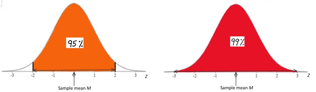
With this approach, we would use the normal distribution’s areas under the curve to figure out the range we need to capture the research population mean with a particular probability. As you can see, the range from a Z-score of -2 to +2 is pretty close to 95% probability, and the range of -3 to +3 is close to 99%. We place the sample mean, calculated from our research study sample, in the middle of this normal distribution. The task, then, is to add either 2 or 3 standard deviations to the mean to find the upper bound, and subtract either 2 or 3 standard deviations to find the lower bound of the confidence interval. How many standard deviations you must go to be sure you include the population mean depends on how confident you need to be. Are you okay with 95% confidence, or should you have 99% confidence? That decision is based on tolerance for Type I error, just like with significance levels in hypothesis testing.

To find precisely the Z-scores matching 95 or 99% confidence intervals, we can use the normal curve areas table. For a 95% confidence interval, just like with a two-tailed hypothesis test with significance level of .05, the Z score that precisely corresponds with 2.5% area in the tails on either side of the curve, or 47.5% area from the mean to the Z score, is Z = 1.96. To find the lower end of the confidence interval, use this formula:

In other words, subtract 1.96 standard deviations from the sample mean. To find the upper end of the interval, use this formula:

In other words, add 1.96 standard deviations to the sample mean. Once you have those two limits, you can make the claim that there is a 95% chance that the research population mean corresponding to this sample mean is between the lower end and the upper end of the confidence interval.

Once you have that range, you can also determine whether there is a statistically significant difference between the research and comparison population mean, by answering this question: does the comparison population mean fall within the reported confidence interval? If so, there is no significant difference. The two means are too close together. If it falls outside the interval, then you can report a significant difference between means.

So you end up at the same place, whether you use hypothesis testing or confidence intervals. The difference is simply in where you start from. Also, hypothesis testing can be one-tailed, but it is uncommon to see directional confidence intervals. Finally, if p-values are reported precisely, hypothesis testing offers slightly more information, but if they are not reported, confidence intervals offer more information. It is a matter of professional preference which technique you choose as a method for making inferences about data following a research study.

Chapter Summary

In this chapter, we covered three big concepts that are vital to understand in the context of inferential statistics. Effect size offers information critical to interpreting a finding of statistical significance. Power tells us whether tests of significance are even worth doing, or if we are at too much risk of Type II error. Confidence intervals offer a system for statistical inference that represents a full alternative to the hypothesis testing procedure we employed for the past several chapters.

Key terms: