8. Analysis of Variance, Planned Contrasts and Posthoc Tests
8a. Analysis of Variance
In this chapter we graduate from teenage statistics to adult statistics! Analysis of Variance is a technique that is very widely used in the analysis of data in psychology and many other disciplines. It is a system of analysis that is very flexible, and it is based on a statistical concept called the general linear model. Once you learn how to use it, you can adapt it to nearly any situation.
Our tasks for this lesson include grasping the concept of partitioning variance into different buckets, like treatment effects vs. error, or between-groups vs. within-groups variance. Next, we will have a look at why Analysis of Variance is needed to analyze data from experimental designs with more than 2 groups. In particular we will examine the dangers of inflating the risk of Type I error, or alpha. And finally, we will demystify the analysis of variance system by conducting a one-way ANOVA. Just to give a little preview, in the following lessons, we will learn how to follow up on ANOVA with planned contrasts and post hoc tests, and then we will progress to a two-way ANOVA with factorial analysis.
The most important concept to grasp in order to intuitively understand what analysis of variance does, is the partitioning of variance. Variance should be a familiar concept by now. Variance is a statistic that summarizes the extent to which the individual scores in a dataset are spread out from the mean. It is calculated by the following steps:
Steps to calculate variance (sample-based estimate for a population)
- Take the distance (“deviation”) of each score from the mean.
- Next, Square each distance to get rid of the sign (because some deviations will be negative).
- Add up all the resulting “squared deviations”. This number is known as “sum of squares” (SS).
- Divide the SS by the number of scores minus 1.
This gives us an estimated variance based on a sample, that is appropriate to use in statistical analysis, in which we want to use the differences between sample means to make inferences about the differences between population means.
The way the partitioning of variance works is this. Differences among scores exist for all sorts of reasons. One of those reasons is the one we are actually interested in. Systematic difference cause by treatments or associated with known characteristics of interest are the differences we are hoping to see in the data. The difference in amount of sleep that can be attributed to the effects of a new drug. The difference in mood specifically caused by chocolate. These are difference between groups, or between samples, that can be explained by the variable of interest.
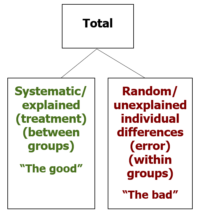
However, there are also difference between scores that are not explained by the variable of interest. These are random, or unsystematic differences. The individual differences among scores within an experimental or control condition count in this category. Error in experimental design or in our measurements also go in this bin. When we want to make an objective decision about data, we need to separate out the systematic, explained differences, which we can label “good variance”, from the random, unexplained differences, which we shall label “bad variance”. Note that good and bad in this context just means it counts toward (“good”) or against (“bad”) statistical significance.
Before we get to numeric examples of partitioning variance, maybe a visual example will help. At left we have a whole sample of dots of various colours.
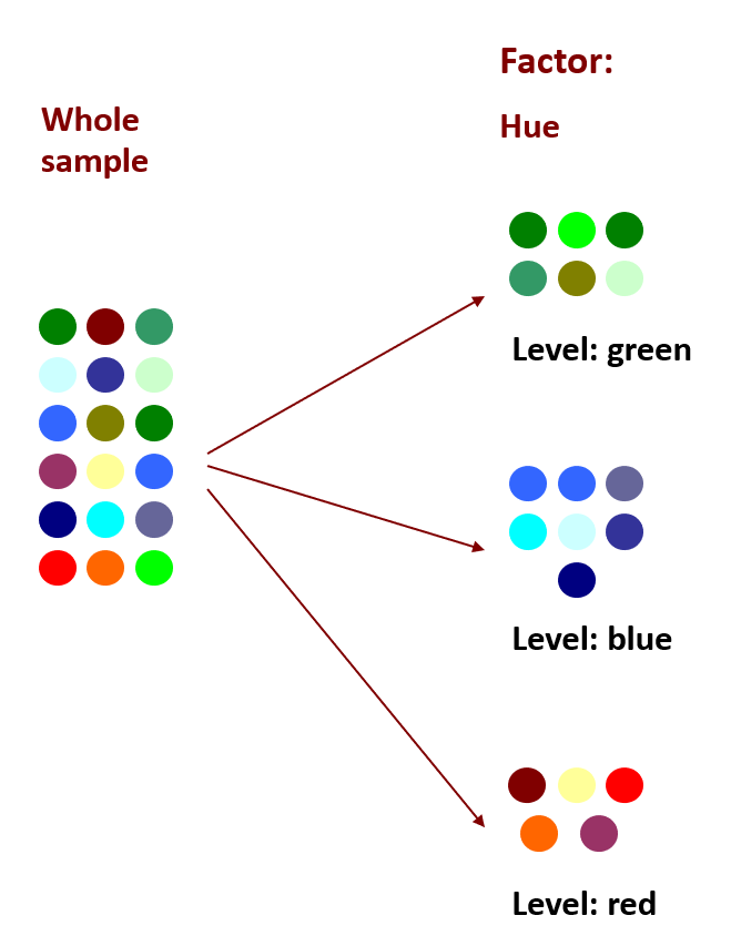
What if we wanted to sort the data by hue, to achieve greater consistency in colour within each group. We can apply the factor of hue to the dots, using three levels: green, blue and red. There are still variations of hue within each grouping, but some of the systematic variability has been separated out by grouping into these three levels. Thus we have accounted for (or explained) some proportion of the variance. The more variance we can explain, the more confident we can be in the effect of our factors. (In an experimental design, factors are independent variables.)
In the next chapter, we will see that applying an additional factor can further sort the colours, to account for even more variability among colours. The more variance we can explain, through multiple factors and/or multiple levels, the better! This is what we will be able to do with two-way ANOVA and factorial designs.
Note: a one-way ANOVA includes one factor, whereas a two-way ANOVA includes two factors.
Think of data analysis as a game in which the goal is to explain as much of the variability in the scores as possible through known factors. It’s like imposing order over chaos in order to see patterns more clearly.
Analysis of Variance becomes necessary when we have experimental designs that are more complex than the ones we have used to date. Up until now, we have covered statistical tests that can handle one-sample and two-sample experimental designs. But what if we are comparing three or more samples? 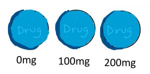 For example, what if we have a drug trial in which we are comparing the mean pain levels of patients after receiving placebo, a low dose of the drug, or a high dose of the drug?
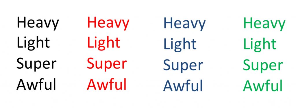 Or what if our memory test using various types of stimuli measures memory for lists of words in black, red, blue or green? ANOVA can handle comparisons among 3, 4, or really any number of groups at once.
Let’s make sure we have a handle on the jargon that is used in ANOVA. First of all, the shortened term ANOVA came from making an acronym of sorts from the phrase Analysis of Variance. Secondly, the term factor is used to designate a nominal variable, or in the case of an experimental design, the independent variable, that designates the groups being compared. If we have a drug trial in which we are comparing the mean pain scores of patients after receiving placebo, a low dose of the drug, or a high dose of the drug, the factor would be “drug dose.” Finally, the term levels refers to the individual conditions or values that make up a factor. In our drug trial example, we have three levels of drug dose: placebo, low dose, and high dose.
So how is this ANOVA thing different from the t-tests we already learned? Well, in fact, you can think of it as an extension of the t-test to more than 2 groups. If you run an ANOVA on just 2 groups, the results are equivalent to the t-test. The only difference is that you get an F-value instead of a t-value. Fun fact – the statistician who invented the t-test published it under a pseudonym “Student”. Perhaps he was scared of the angst of the many students who would have to learn to use it. The F-test, however, is named for Fisher. He apparently had no such fear. Maybe he was that confident that students would love learning ANOVA. Hopefully he was right… ! Anyway, trust me – if you were to calculate the t-value and the F-value for the exact same two sample, the F-value would be the t-value squared.
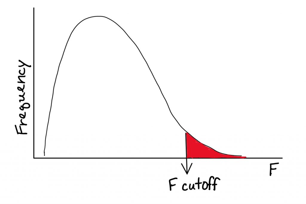
There is a nice part of using the F distribution and a not so nice part of it. The F distribution requires two degrees of freedom. Annoying, yes. But the nice part outweighs that annoyance, in my opinion. The F distribution starts from 0 and heads to the right. It has only positive values.
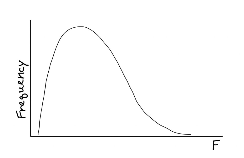
What this means is no more distribution sketches, and no more one-tailed or two-tailed nonsense. So the logistics of the hypothesis test actually get a whole lot simpler.
You might be wondering, okay so the ANOVA thing has some advantages, but we do already know the t-test, so could we not just use multiple t-tests to compare each group within the factor against each other? The problem is, each comparison includes a risk of a Type I error. The risk of Type I error accumulates with multiple statistical tests on the same data, and that is called the experimentwise alpha level. ANOVA does one overall, or omnibus, test of treatment effects, to keep our risk of Type I error down. Inflating alpha is dangerous, and any statistical method we can use to keep it under control is a good thing.
The calculation method I will show you differs from more efficient methods you can find on the internet or in many other textbooks. Sorry for that, but the nice thing about the method I will show you here is that it has beautiful symmetry to it and highlights the concept of partitioning of variance. In other words these are conceptual rather than calculational formulas. This is a deliberate choice to help you understand how ANOVA works, because if we think about it, you will never need to calculate statistics by hand in the “real world.” You will always be able to use a computer instead. However, all the computers in the world cannot help you choose an appropriate statistic for a particular situation, or to understand/articulate how the selected statistical test works. This is what an introduction to statistics is really about.
There will also be an inherent math double-check opportunity in this method, which I think you will appreciate. In reality, most people use a computer to calculate ANOVA. However, I do like to ask you to try calculating things by hand, so you can see how it works. My hope is that you gain a better conceptual understanding of the mechanisms behind these statistical tests by applying them, and seeing how it all fits together like a puzzle, with tangible examples. Given that, I think this calculation system is better than others you can use.
So, how does ANOVA work? Essentially it works by calculating different kinds of Sums of squares, which we will continue to abbreviate as SS. As you can see, there are three flavours of SS that can each be calculated using the formulas shown.
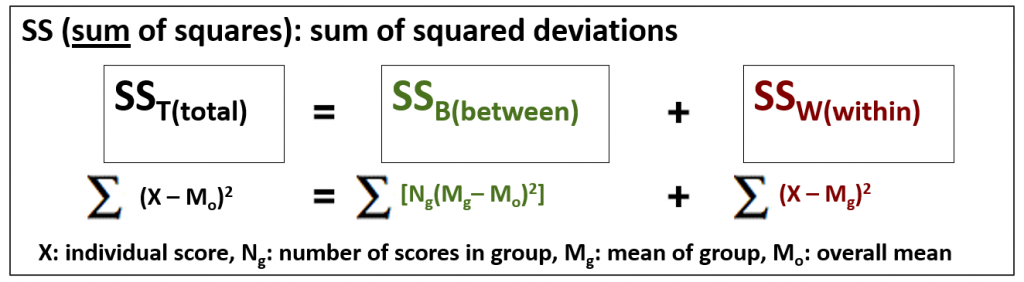
The Sum of squares Between-groups (SSB) and Sum of Squares Within-groups (SSW) should add up to the Sum of Squares Total (SST). So here you see the partitioning of variance coming in.
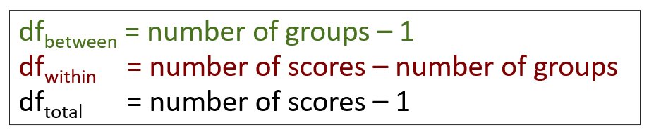
There are also three flavours of degrees of freedom, with matching labels. They also should add up.
Notice I used colour coding to help you track the “good” variance in green and the “bad” variance in red.
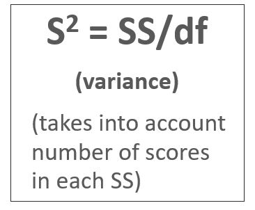
Once you have the SS and degrees of freedom calculated, you can find the variances.
The F-test is simple: it is the ratio of explained to unexplained variance, which is represented by the variance between and the variance within. You need more explained than unexplained variance to be able to reject the null.
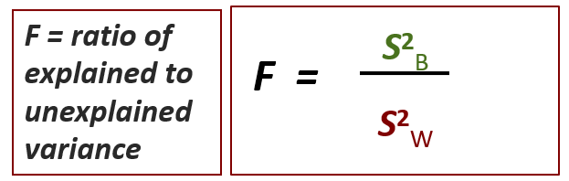
How much the ratio needs to be depends on the degrees of freedom. And that’s where sample size becomes very important, just as we saw in the t-test.
One of the beautiful things about ANOVA is the calculation table. This is a way of organizing all the components of the workflow, and also highlighting our two math double-checks. For both SS and degrees of freedom, the Between and Within numbers should add up to the total.
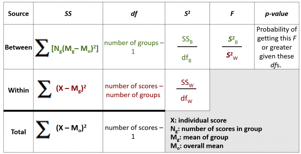
This table is a good reference for you to keep to hand, as a reminder of each formula and how the ANOVA puzzle fits together.
Note what each symbol in these formulas means, by referring to the symbols key in the lower right of the table. The one element that tends to be confusing is Ng. This symbol refers to the number of scores in the group – not to the number of groups in the study. This is important to interpret correctly. If you ever find that your SSB and SSW do not add up to your SST, like really not even close, then that is the first thing to double check. Did you use the number of scores in the group when calculating SSB?
Now that our research designs are getting more complex, our statistical findings will need a little more descriptive statistics and graphical portrayal in order to easily interpret what those hypothesis test results really tell us. I would encourage you to always graph the means and standard deviations of your data before conducting your inferential statistics, so that you get a sense for significance before you begin. Do not go blind into that statistical routine… remember, numbers are never as informative as a picture of the data.
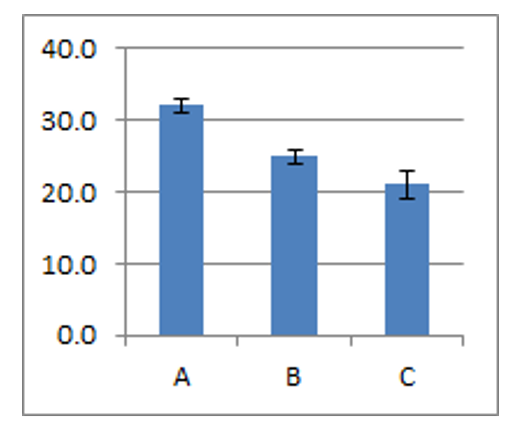
I recommend a bar graph displaying group means, and adding error bars as tall as the standard deviation (or standard error) on top of the mean. You can also show the bars going one standard deviation downward as well, to get the full range of the typical scores in the group.
If the error bars eclipse the difference in group means, that is a bad sign if your goal is to report a significant difference among means. This visual allows you to preview the signal-to-noise ratio in your data, or your between-to-within variance ratio.
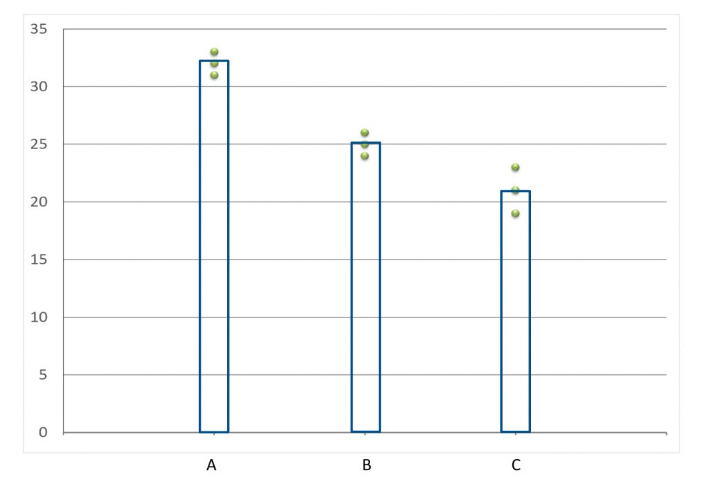 Another really great visual is the group scatter plot, shown here. It is not really a standard way to view datasets, but I think it should be.
Step 1 of hypothesis testing for an ANOVA truly becomes a formality. The hypotheses are always the same. Define a population for each group. Set the research hypothesis to be a general statement of difference among population means. Set the null to be a statement of equality among population means. There is no directionality with the F distribution, so we do not need to worry about the predicted direction of differences.
Using our drug-dose example with three levels, the populations and hypotheses would look something like this:
![]() Now we can move on to step 2. The F distribution has two degrees of freedom.
Now we can move on to step 2. The F distribution has two degrees of freedom.
We no longer have to worry about the mean or standard deviation of the comparison distribution, we just need to find the degrees of freedom between and within. The “good” variance is the differences between groups, and so the degrees of freedom between is number of groups – 1. The within-groups variance, the “bad” variance, is the individual differences among the scores within each group. The degrees of freedom within, then, is the total number of scores in all groups, minus the number of groups.
For step 3, we can find the cutoff score in the F-tables if we know the significance level, degrees of freedom between and degrees of freedom within.
Step 4 is where things take some getting used to. Here we use this new system of formulas. Start with Sum of squares calculations: Between, Within, and Total, and double check that both they and the degrees of freedom add up.
![\[SS_{B}=\sum [N_{g}(M_{g}-M_{o})^{2}]\]](https://pressbooks.bccampus.ca/statspsych/wp-content/ql-cache/quicklatex.com-658f4be8fa5ebfc693cd4b836f659c25_l3.png "Rendered by QuickLaTeX.com")
![\[SS_{W}=\sum (X-M_{g})^{2}\]](https://pressbooks.bccampus.ca/statspsych/wp-content/ql-cache/quicklatex.com-310d82aa6481cef324934a3fe5919060_l3.png "Rendered by QuickLaTeX.com")
![\[SS_{T}=\sum (X-M_{o})^{2}\]](https://pressbooks.bccampus.ca/statspsych/wp-content/ql-cache/quicklatex.com-e2b80b3aae3459a94014ca3cd2a4b153_l3.png "Rendered by QuickLaTeX.com")
Then move across the table, finding the good and the bad variance…
![\[S^{2}_{B}=\frac{SS_{B}}{df_{B}}\]](https://pressbooks.bccampus.ca/statspsych/wp-content/ql-cache/quicklatex.com-94ac068d1f6fa970b59d402068ee0878_l3.png "Rendered by QuickLaTeX.com")
![\[S^{2}_{W}=\frac{SS_{W}}{df_{W}}\]](https://pressbooks.bccampus.ca/statspsych/wp-content/ql-cache/quicklatex.com-e5fe2424674d311235f0a59ef07afcc6_l3.png "Rendered by QuickLaTeX.com")
… and finally getting their ratio for the F-test result.
![\[F=\frac{S^{2}_{B}}{S^{2}_{W}}\]](https://pressbooks.bccampus.ca/statspsych/wp-content/ql-cache/quicklatex.com-10eb2646ad2196e5dcf5ec027e2f3e7d_l3.png "Rendered by QuickLaTeX.com")
To make our decision in Step 5, we examine the calculated F value (from Step 4) and determine whether it exceeds the cutoff F score (from Step 3). If so, we reject the null hypothesis.
“There is a significant difference among the mean digit memory scores after listening to the three types of music (f2,6 = 27.00, p < 0.05).” Here is an example of how to express the results – note the phrase “significant difference among the means.” If we do not reject the null, we can switch the statement of results to “no significant difference.” The test statistic and p-values are expressed here in common formats.
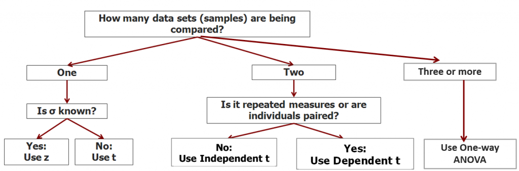
We can continue building a decision tree to help you decide which statistical test to use when you look at a research question. What are the circumstances in which you would need to use a one-way ANOVA test?
8b. Planned Contrasts and Posthoc Tests
In the second part of this chapter we will have a look at follow-up tests we can conduct after an ANOVA hypothesis test, to investigate the findings in greater detail.
Planned contrasts and post-hoc tests are commonly performed following Analysis of Variance. This is necessary in many instances, because ANOVA compares all individual mean differences simultaneously, in one test (referred to as an omnibus test). If we run an ANOVA hypothesis test, and the F-test comes out significant, this indicates that at least one among the mean differences is statistically significant. However, when the factor has more than two levels, it does not indicate which means differ significantly from each other.
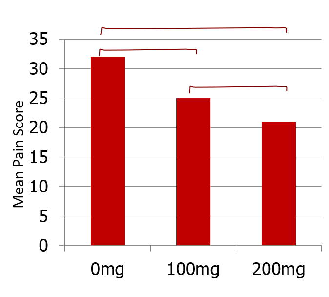
In this example, a significant F-test result from a one-way ANOVA with the three drug dose conditions does not tell us where the significant difference lies. Is it between 0 and 100 mg? Or between 100 and 200 mg? Or is it only the biggest difference that is significant – 0 vs. 200 mg?
Planned contrasts and post hoc tests are additional tests to determine exactly which mean differences are significant, and which are not. Why is that we cannot just do 3 independent means t-tests here? Each time we conduct a t-test we have a certain risk of a Type I error. If we do 3, we have triple the risk. So first we test for omnibus significance using the overall ANOVA as detailed in the first part of this chapter. Then, if a statistically significant difference exists among the means, we do the pairwise comparisons with an adjustment to be more conservative. These follow-up tests are designed specifically to avoid inflating risk of Type I error.
Now, this is very important. We are only allowed to conduct these tests if the F-test result was significant. This procedural rule also helps protect us from the statistical sin of p-hacking, which is selectively hunting for and reporting significant results in a way that is biased and subjective.
Planned contrasts are used when researchers know in advance which groups they expect to differ. For example, suppose from our worksheet example, we expect the pop group to differ from the classical group on our measure of working memory. We can then conduct a single comparison between these means without worrying about Type I error. Because we hypothesized this difference before we saw the data, perhaps based on prior research studies or a strong intuitive hunch, and because there is only one comparison to be analyzed, we need not be concerned about inflated experimentwise alpha. If multiple comparisons are planned, then we will need to adjust the significance level.
Let us take a look at how to conduct a single planned contrast. The process is quite simple, as it is just a modified ANOVA analysis. First we calculate SSB with just those two groups involved in the planned contrast. We figure out the degrees of freedom between using just the two groups. Then, we calculate the variance between using the new SSB and degrees of freedom, and we calculate an F-test for the comparison using the new variance between and the original overall variance within. To find out if the F-test result is significant, we can use the new degrees of freedom but the original significance level for the cutoff. (Because there is just one pairwise comparison, we can use original significance level.)
Steps to calculate a planned contrast
- Calculate SSBetween with just those two groups.
- Find the dfBetween using just the two groups.
- Calculate S2Between using the new SSBetween and the new dfBetween.
- Calculate F using the new S2Between and the overall S2Within.
If we were to perform multiple planned contrasts, things change a little. Suppose we had hypothesized in this experiment that each group would differ from the others? The Bonferroni correction involves adjusting the significance level to protect from the inflation of risk of Type I error. The procedure for each comparison is the same as for a single planned contrast. The difference is that the cutoff score to determine statistical significance will use a more conservative significance level. When we do multiple pairwise comparisons, the Bonferroni correction is to use the original significance level divided by number of planned contrasts. The adjusted significance level is not likely to be in our F-tables, so to find the cutoff for such tests, we would need to use an online calculator in reverse (that is, we enter the p-value and degrees of freedom, and look up the value on the F-distribution corresponding to that area in the tail).
What about post hoc tests tests? As the name suggests, these tests come into the picture when we are doing pairwise comparisons (usually all possible combinations) after the fact to find out where the significant differences were. These are tests that do not require that we had an a priori hypothesis ahead of data collection. Essentially, these are an allowable and acceptable form of data-snooping. This is where we must be cautious about doing so many tests – we could end up with huge risk of Type I error. If we use the Bonferroni correction that we saw for multiple planned comparisons on more than 3 tests, the significance level would be vanishingly small. This would make it nearly impossible to detect significant differences. For this reason, slightly more forgiving tests like Scheffe’s correction, Dunn’s or Tukey’s post-hoc tests are more popular. There are many different post-hoc tests out there, and the choice of which one researchers use is often a matter of convention in their area of research.
Now we shall take a look at how to conduct post hoc tests using Scheffé’s correction. In this example, we will test all pairwise comparisons. The Scheffé technique involves adjusting the F-test result, rather than adjusting the significance level. The way it works is the same as the planned contrast procedure, except for the very end. Before we compare the F-test result to the cutoff score, we divide the F value by the overall degrees of freedom between, or the number of groups minus one. Thus, we keep the significance level at the original level, but divide the calculated F by overall degrees of freedom between from the overall ANOVA.
Steps to calculate post-hoc tests with Scheffé’s correction
For each pairwise comparison:
- Calculate SSBetween with just those two groups.
- Find the dfBetween using just the two groups.
- Calculate S2Between using the new SSBetween and the new dfBetween.
- Calculate F using the new S2Between and the overall S2Within.
- Divide F by overall dfBetween.
Chapter Summary
In this chapter we introduced the concepts underlying Analysis of Variance and examined how to conduct a hypothesis test using this technique. We also saw how to follow up on a statistically significant F-test result in an ANOVA with more than two levels in a factor, in order to determine which levels were significantly different from each other.
Key terms:
| Analysis of Variance | post hoc tests | Bonferroni correction |
| general linear model | factor | Scheffé correction |
| partitioning of variance | levels | |
| planned contrasts | experimentwise alpha level | |
also called ANOVA, a system of data analysis that is very flexible and adaptable to a variety of research designs. It is based on a statistical concept called the general linear model and involves the technique of partitioning variance.
an extension of the statistical technique linear regression that is adaptable to various combinations of independent (nominal) and dependent (numeric) variables
the allocation of variability among scores in numeric data into different buckets, like treatment effects vs. error, or between-groups vs. within-groups variance
statistical tests of pairwise comparisons among groups, used to follow up on a significant ANOVA result, when researchers know in advance which groups they expect to differ
statistical tests of pairwise comparisons among groups, used to follow up on a significant ANOVA result, when researchers do not know in advance which groups they expect to differ and wish to test all possible combinations
in ANOVA, a grouping variable used to account for variance among scores; in an experiment a factor is an independent variable
the individual conditions or values that make up a factor, a nominal variable that forms the groups in analysis of variance
the problem of accumulating risk of Type I error with multiple statistical tests on the same data
adjustment to avoid inflation of experimentwise risk of Type I error, by dividing significance level by the number of planned contrasts to be conducted
in posthoc analyses, an adjustment to correct for inflated experimentwise risk of Type I error, by dividing the F value by the overall degrees of freedom between from the original overall ANOVA analysis
