4. Probability, Inferential Statistics, and Hypothesis Testing
4a. Probability and Inferential Statistics
video lesson
In this chapter, we will focus on connecting concepts of probability with the logic of inferential statistics.
“The whole problem with the world is that fools and fanatics are always so certain of themselves, and wiser people so full of doubts.”
— Bertrand Russel (1872-1970)
These notable quotes represent why probability is critical for a basic understanding of scientific reasoning.
“Medicine is a science of uncertainty and an art of probability.”
— William Osler (1849–1919)In many ways, the process of postsecondary education is all about instilling a sense of doubt and wonder, and the ability to estimate probabilities. As a matter of fact, that essentially sums up the entire reason why you are in this course. So let us tackle probability.
We will be keeping our coverage of probability to a very simple level, because the introductory statistics we will cover rely on only simple probability. That said, I encourage you to read further on compound and conditional probabilities, because they will certainly make you smarter at real-life decision making. We will briefly touch on examples of how bad people can be at using probability in real life, and we will then address what probability has to do with inferential statistics. Finally, I will introduce you to the central limit theorem. This is probably one of the heftiest math concepts in the course, but worry not. Its implications are easy to learn, and the concepts behind it can be demonstrated empirically in the interactive exercises.
First, we need to define probability. In a situation where several different outcomes are possible, the probability of any specific outcome is a fraction or proportion of all possible outcomes. Another way of saying that is this. If you wish to answer the question, “What are the chances that outcome would have happened?”, you can calculate the probability as the ratio of possible successful outcomes to all possible outcomes.
Concept Practice: define probability
People often use the rolling of dice as examples of simple probability problems.

If you were to roll one typical die, which has a number on each side from 1 to 6, then the simple probability of rolling a 1 would be 1/6. There are six possible outcomes, but only 1 of them is the successful outcome, that of rolling a 1.
Concept Practice: calculate probability
Another common example used to introduce simple probability is cards. In a standard deck of casino cards, there are 52 cards. There are 4 aces in such a deck of cards (Aces are the “1” card, and there is 1 in each suit – hearts, spades, diamonds and clubs.)

If you were to ask the question “what is the probability that a card drawn at random from a deck of cards will be an ace?”, and you know all outcomes are equally likely, the probability would be the ratio of the number of times one could draw and ace divided by the number of all possible outcomes. In this example, then, the probability would be 4/52. This ratio can be converted into a decimal: 4 divided by 52 is 0.077, or 7.7%. (Remember, to turn a decimal to a percent, you need to move the decimal place twice to the right.)
Concept Practice: calculate probability
Probability seems pretty straightforward, right? But people often misunderstand probability in real life. Take the idea of the lucky streak, for example. Let’s say someone is rolling dice and they get 4 6’s in a row. Lots of people might say that’s a lucky streak and they might go as far as to say they should continue, because their luck is so good at the moment! According to the rules of probability, though, the next die roll has a 1/6 chance of being a 6, just like all the others. True, the probability of a 4-in-a-row streak occurring is fairly slim: 1/6 x 1/6 x 1/6 x 1/6. But the fact is that this rare event does not predict future events (unless it is an unfair die!). Each time you roll a die, the probability of that event remains the same. That is what the human brain seems to have a really hard time accepting.
Concept Practice: lucky streak
When someone makes a prediction attached to a certain probability (e.g. there is only a 1% chance of an earthquake in the next week), and then that event occurs in spite of that low probability estimate (e.g. there is actually an earthquake the day after the prediction was made)… was that person wrong? No, not really, because they allowed for the possibility. Had they said there was a 0% chance, they would have been wrong.
Probabilities are often used to express likelihood of outcomes under conditions of uncertainty. Like Bertrand Russell said, wise people rarely speak in terms of certainties. Because people so often misunderstand probability, or find irrational actions so hard to resist despite some understanding of probability, decision making in the realm of sciences needs to be designed to combat our natural human tendencies. What we are discussing now in terms of how to think about and calculate probabilities will form a core component of our decision-making framework as we move forward in the course.
Now, let’s take a look at how probability is used in statistics.
Concept Practice: area under normal curve as probability
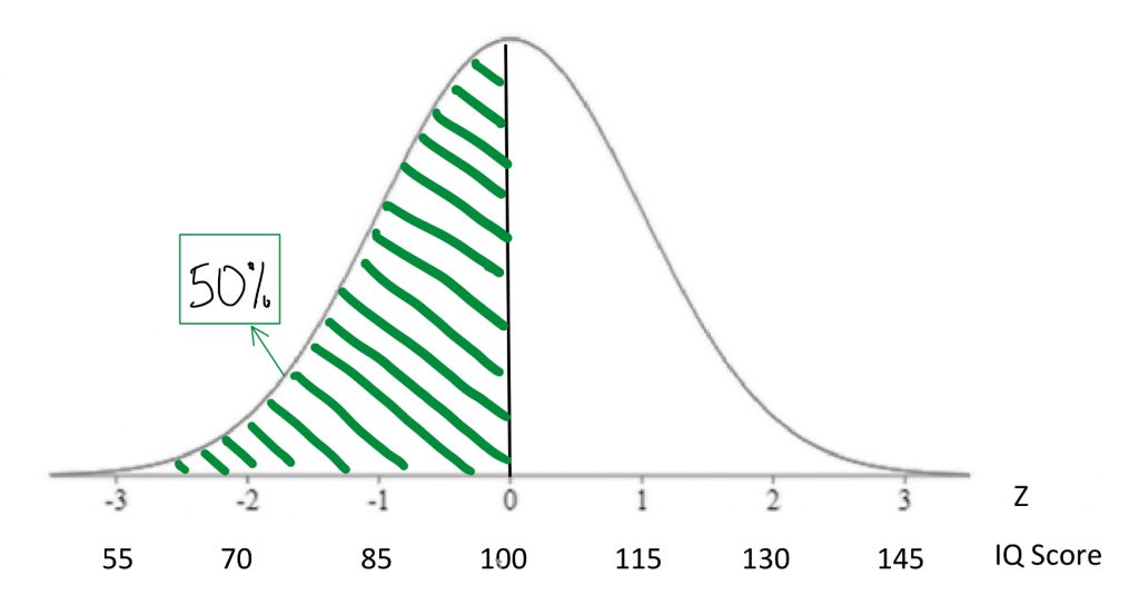
We saw that percentiles are expressions of area under a normal curve. Areas under the curve can be expressed as probability, too. For example, if we say the 50th percentile for IQ is 100, that can be expressed as: “If I chose a person at random, there is a 50% chance that they will have an IQ score below 100.”
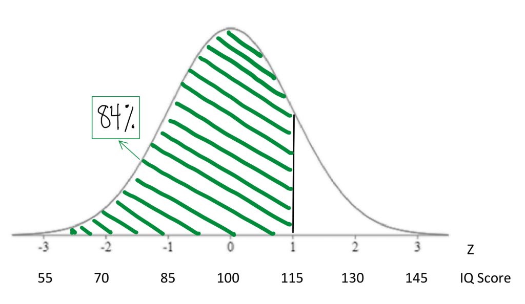
If we find the 84th percentile for IQ is 115 there is another way to say that “If I chose a person at random, there is an 84% chance that they will have an IQ score below 115.”
Concept Practice: find percentiles
Any time you are dealing with area under the normal curve, I encourage you to express that percentage in terms of probabilities. That will help you think clearly about what that area under the curve means once we get into the exercise of making decisions based on that information.
Concept Practice: interpreting percentile as probability
Probabilities, of course, range from 0 to 1 as proportions or fractions, and from 0% to 100% when expressed in percentage terms. In inferential statistics, we often express in terms of probability the likelihood that we would observe a particular score under a given normal curve model.
Concept Practice: applying probability
Although I encourage you to think of probabilities as percentages, the convention in statistics is to report to the probability of a score as a proportion, or decimal. The symbol used for “probability of score” is p. In statistics, the interpretation of “p” is a delicate subject. Generations of researchers have been lazy in our understanding of what “p”: tells us, and we have tended to over-interpret this statistic. As we begin to work with “p”, I will ask you to memorize a mantra that will help you report its meaning accurately. For now, just keep in mind that most psychologists and psychology students still make mistakes in how they express and understand the meaning of “p” values. This will take time and effort to fix, but I am confident that your generation will learn to do better at a precise and careful understanding of what statistics like “p” tell us… and what they do not.
To give you a sense of what a statement of p < .05 might mean, let us think back to our rat weights example.
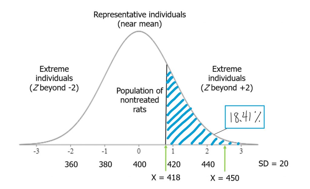
If I were to take a rat from our high-grain food group and place it on the distribution of untreated rat weights, and if it placed at Z = .9, we could look at the area under the curve from that point and above. That would tell us how likely it would be to observe such a heavy rat in the general population of nontreated rats — those that eat a normal diet.
Think of it this way. When we select a rat from our treatment group (those that ate the grain-heavy diet), and it is heavier than the average for a nontreated rat, there are two possible explanations for that observation. One is that the diet made him that way. As a scientist whose hypothesis is that a grain-heavy diet will make the rats weigh more, I’m actually motivated to interpret the observation that way. I want to believe this event is meaningful, because it is consistent with my hypothesis! But the other possibility is that, by random chance, we picked a rat that was heavy to begin with. There are plenty of rats in the distribution of nontreated rats that were at least that heavy. So there is always some probability that we just randomly selected a heavier rat. In this case, if my treated rat’s weight was less than one standard deviation above the mean, we saw in the chapter on normal curves that the probability of observing a rat weight that high or higher in the nontreated population was about 18%. That is not so unusual. It would not be terribly surprising if that outcome were simply the result of random chance rather than a result of the diet the rat had been eating.
If, on the other hand, the rat we measured was 2.5 standard deviations above the mean, the tail probability beyond that Z-score would be vanishingly small.
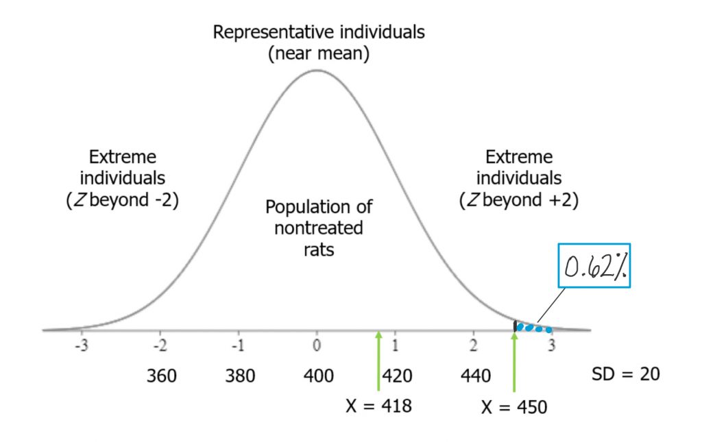
The probability of observing such a rat weight in the nontreated population is very low, so it is far less likely that observation can be accounted for just by random chance alone. As we accumulate more evidence, the probability they could have come at random from the nontreated population will weigh into our decision making about whether the grain-heavy diet indeed causes rats to become heavier. This is the way probabilities are used in the process of hypothesis testing, the logic of inferential statistics that we will look at soon.
Concept Practice: statistics as probability
Now that you have seen the relevance of probability to the decision making process that comprises inferential statistics, we have one more major learning objective: to become familiar with the central limit theorem.
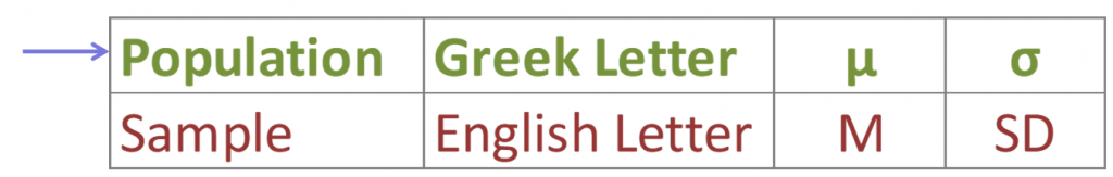
However, before we get to the central limit theorem, we need to be clear on the distinction between two concepts: sample and population. In the world of statistics, the population is defined as all possible individuals or scores about which we would ideally draw conclusions. When we refer to the characteristics, or parameters, that describe a population, we will use Greek letters. A sample is defined as the individuals or scores about which we are actually drawing conclusions. When we refer to the characteristics, or statistics, that describe a sample, we will use English letters.
It is important to understand the difference between a population and a sample, and how they relate to one another, in order to comprehend the central limit theorem and its usefulness for statistics. From a population we can draw multiple samples. The larger sample, the more closely our sample will represent the population.
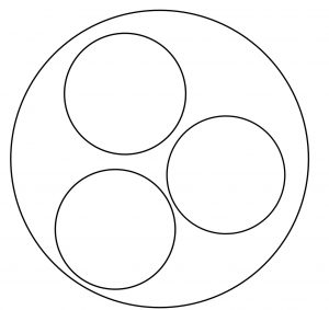
Think of a Venn diagram. There is a circle that is a population. Inside that large circle, you can draw an infinite number of smaller circles, each of which represents a sample.
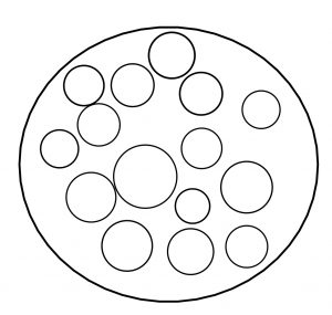
The larger that inner circle, the more of the population it contains, and thus the more representative it is.
Let us take a concrete example. A population might be the depression screening scores for all current postsecondary students in Canada. A sample from that population might be depression screening scores for 500 randomly selected postsecondary students from several institutions across Canada. That seems a more reasonable proportion of the two million students in the population than a sample that contains only 5 students. The 500 student sample has a better shot at adequately representing the entire population than does the 5 student sample, right? You can see that intuitively… and once you learn the central limit theorem, you will see the mathematical demonstration of the importance of sample size for representing the population.
To conduct the inferential statistics we are using in this course, we will be using the normal curve model to estimate probabilities associated with particular scores. To do that, we need to assume that data are normally distributed. However, in real life, our data are almost never actually a perfect match for the normal curve.
So how can we reasonably make the normality assumption? Here’s the thing. The central limit theorem is a mathematical principle that assures us that the normality assumption is a reasonable one as long as we have a decent sample size.
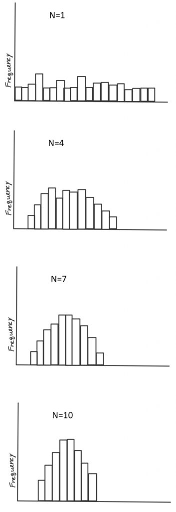
According to the theorem, as long as we take a decent-sized sample, if we took many samples (10,000) of large enough size (30+) and took the mean each time, the distribution of those means will approach a normal distribution, even if the scores from each sample are not normally distributed. To see this for yourself, take a look at the histograms shown on the right. The top histogram came from taking from a population 10,000 samples of just one score each, and plotting them on a histogram. See how it has a flat, or rectangular shape? No way we could call that a shape approximating a normal curve. Next is a histogram that came from taking the means of 10,000 samples, if each sample included 4 scores. Looks slightly better, but still not very convincing. With a sample size of 7, it looks a bit better. Once our sample size is 10, we at least have something pretty close. Mathematically speaking, as long as the sample size is no smaller than 30, then the assumption of normality holds. The other way we can reasonably make the normality assumption is if we know the population itself follows a normal curve. In that case, even if individual samples do not have a nice shaped histogram, that is okay, because the normality assumption is one apply to the population in question, not to the sample itself.
Now, you can play around with an online demonstration so you can really convince yourself that the central limit theorem works in practice. The goal here is to see what sample size is sufficient to generate a histogram that closely approximates a normal curve. And to trust that even if real-life data look wonky, the normal curve may still be a reasonable model for data analysis for purposes of inference.
Concept Practice: Central Limit Theorem
4b. Hypothesis Testing
video lesson
We are finally ready for your first introduction to a formal decision making procedure often used in statistics, known as hypothesis testing.
In this course, we started off with descriptive statistics, so that you would become familiar with ways to summarize the important characteristics of datasets. Then we explored the concepts standardizing scores, and relating those to probability as area under the normal curve model. With all those tools, we are now ready to make something!

Okay, not furniture, exactly, but decisions.
We are now into the portion of the course that deals with inferential statistics. Just to get you thinking in terms of making decisions on the basis of data, let us take a slightly silly example. Suppose I have discovered a pill that cures hangovers!

Well, it greatly lessened symptoms of hangover in 10 of the 15 people I tested it on. I am charging 50 dollars per pill. Will you buy it the next time you go out for a night of drinking? Or recommend it to a friend? … If you said yes, I wonder if you are thinking very critically? Should we think about the cost-benefit ratio here on the basis of what information you have? If you said no, I bet some of the doubts I bring up popped to your mind as well. If 10 out of 15 people saw lessened symptoms, that’s 2/3 of people – so some people saw no benefits. Also, what does “greatly lessened symptoms of hangover” mean? Which symptoms? How much is greatly? Was the reduction by two or more standard deviations from the mean? Or was it less than one standard deviation improvement? Given the cost of 50 dollars per pill, I have to say I would be skeptical about buying it without seeing some statistics!
On this list is a preview of the basic concepts to which you will be introduced as we go through the rest of this chapter.
Hypothesis Testing Basic Concepts
- Hypothesis
- Null Hypothesis
- Research Hypothesis (alternative hypothesis)
- Statistical significance
- Conventional levels of significance
- Cutoff sample score (critical value)
- Directional vs. non-directional hypotheses
- One-tailed and two-tailed tests
- Type I and Type II errors
You can see that there are lots of new concepts to master. In my experience, each concept makes the most sense in context, within its place in the hypothesis testing workflow. We will start with defining our null and research hypotheses, then discuss the levels of statistical significance and their conventional usage. Next, we will look at how to find the cutoff sample score that will form the critical value for our decision criterion. We will look at how that differs for directional vs. non-directional hypotheses, which will lend themselves to one- or two-tailed tests, respectively.
The hypothesis testing procedure, or workflow, can be broken down into five discrete steps.
Steps of Hypothesis Testing
- Restate question as a research hypothesis and a null hypothesis about populations.
- Determine characteristics of the comparison distribution.
- Determine the cutoff sample score on the comparison distribution at which the null hypothesis should be rejected.
- Determine your sample’s score on the comparison distribution.
- Decide whether to reject the null hypothesis.
These steps are something we will be using pretty much the rest of the semester, so it is worth memorizing them now. My favourite approach to that is to create a mnemonic device. I recommend the following key words from which to form your mnemonic device: hypothesis, characteristics, cutoff, score, and decide. Not very memorable? Try association those with more memorable words that start with the same letter or sound. How about “Happy Chickens Cure Sad Days.” Or you can put the words into a mnemonic device generator on the internet and get something truly bizarre. I just tried one and got “Hairless Carsick Chewbacca Slapped Demons”. Another good one: “Hamlet Chose Cranky Sushi Drunkenly.” Anyway, you play around with it or brainstorm until you hit upon one that works for you. Who knew statistics could be this much fun!
The first step in hypothesis testing is always to formulate hypotheses. The first rule that will help you do so correctly, is that hypotheses are always about populations. We study samples in order to make conclusions about populations, so our predictions should be about the populations themselves. First, we define population 1 and population 2. Population 1 is always defined as people like the ones in our research study, the ones we are truly interested in. Population 2 is the comparison population, the status quo to which we are looking to compare our research population. Now, remember, when referring to populations, we always use Greek letters. So if we formulate our hypotheses in symbols, we need to use Greek letters.
It is a good idea to state our hypotheses both in symbols and in words. We need to make them specific and disprovable. If you follow my tips, you will have it down with just a little practice.
We need to state two hypotheses. First, we state the research hypothesis, which is sometimes referred to as the alternative hypothesis. The research hypothesis (often called the alternative hypothesis) is a statement of inequality, or that Something happened! This hypothesis makes the prediction that the population from which the research sample came is different from the comparison population. In other words, there is a really high probability that the sample comes from a different distribution than the comparison one.
The null hypothesis, on the other hand, is a statement of equality, or that nothing happened. This hypothesis makes the prediction that the population from which sample came is not different from the comparison population. We set up the null hypothesis as a so-called straw man, that we hope to tear down. Just remember, null means nothing – that nothing is different between the populations.
Step two of hypothesis testing is to determine the characteristics of the comparison distribution. This is where our descriptive statistics, the mean and standard deviation, come in. We need to ensure our normal curve model to which we are comparing our research sample is mapped out according to the particular characteristics of the population of comparison, which is population 2.
Next it is time to set our decision rule. Step 3 is to determine the cutoff sample score, which is derived from two pieces of information. The first is the conventional significance level that applies. By convention, the probability level that we are willing to accept as a risk that the score from our research sample might occur by random chance within the comparison distribution is set to one of three levels: 10%, 5%, or 1%. The most common choice of significance level is 5%. Typically the significance level will be provided to you in the problem for your statistics courses, but if it is not, just default to a significance level of .05. Sometimes researchers will choose a more conservative significance level, like 1%, if they are particularly risk averse. If the researcher chooses a 10% significance level, they are likely conducting a more exploratory study, perhaps a pilot study, and are not too worried about the probability that the score might be fairly common under the comparison distribution.
The second piece of information we need to know in order to find our cutoff sample score is which tail we are looking at. Is this a directional hypothesis, and thus one-tailed test? Or a non-directional hypothesis, and thus a two-tailed test? This depends on the research hypothesis from step 1. Look for directional keywords in the problem. If the researcher prediction involves words like “greater than” or “larger than”, this signals that we should be doing a one-tailed test and that our cutoff sample score should be in the top tail of the distribution. If the researcher prediction involves words like “lower than” or “smaller than”, this signals that we should be doing a one-tailed test and that our cutoff sample score should be in the bottom tail of the distribution. If the prediction is neutral in directionality, and uses a word like “different”, that signals a non-directional hypothesis. In that case, we would need to use a two-tailed test, and our cutoff scores would need to be indicated on both tails of the distribution. To do that, we take our area under the curve, which matches our significance level, and split it into both tails.
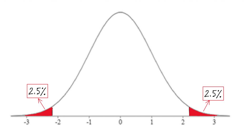
For example, if we have a two-tailed test with a .05 significance level, then we would split the 5% area under the curve into the two tails, so two and a half percent in each tail.
Concept Practice: deciding on one-tailed vs. two-tailed tests
We can find the Z-score that forms the border of the tail area we have identified based on significance level and directionality by looking it up in a table or an online calculator. I always recommend mapping this cutoff score onto a drawing of the comparison distribution as shown above. This should help you visualize the setup of the hypothesis test clearly and accurately.
Concept Practice: inference through hypothesis testing
The next step in the hypothesis testing procedure is to determine your sample’s score on the comparison distribution. To do this, we calculate a test statistic from the sample raw score, mark it on the comparison distribution, and determine whether it falls in the shaded tail or not. In reality, we would always have a sample with more than one score in it. However, for the sake of keeping our test statistic formula a familiar one, we will use a sample size of one. We will use our Z-score formula to translate the sample’s raw score into a Z-score – in other words, we will figure out how many standard deviations above or below the comparison distribution’s mean the sample score is.
![\[Z=\frac{X-M}{SD}\]](https://pressbooks.bccampus.ca/statspsych/wp-content/ql-cache/quicklatex.com-9ff4a1c7099641ee0b6856dfdc537f34_l3.png "Rendered by QuickLaTeX.com")
Finally, it’s time to decide whether to reject the null hypothesis. This decision is based on whether our sample’s data point was more extreme than the cutoff score, in other words, “did it fall in the shaded tail?” If the sample score is more extreme than the cutoff score, then we must reject the null hypothesis. Our research hypothesis is supported! (Not proven… remember, there is still some probability that that score could have occurred randomly within the comparison distribution.) But it is sound to say that it appears quite likely that the population from which our sample came is different from the comparison population. Another way to express this decision is to say that the result was statistically significant, which is to say that there is less than a 5% chance of this result occurring randomly within the comparison distribution (here I just filled in the blank with the significance level).
What if the research sample score did not fall in the shaded tail? In the case that the sample score is less extreme than the cutoff score, then our research hypothesis is not supported. We do not reject the null hypothesis. It appears that the population from which our sample came is not different from the comparison population. Note that we do not typically express this result as “accept the null hypothesis” or “we have proved the null hypothesis”. From this test, we do not have evidence that the null hypothesis is correct, rather we simply did not have enough evidence to reject it. Another way to express this decision is to say that the result was not statistically significant, which is to say that there is more than a 5% chance of this result occurring randomly within the comparison distribution (here I just used the most common significance level).
Concept Practice: interpreting conclusions of hypothesis tests
So we have described the hypothesis testing process from beginning to end. The whole process of null hypothesis testing can feel like pretty tortured logic at first. So let us zoom out, and look at the whole process another way. Essentially what we are seeking to do in such a hypothesis test is to compare two populations. We want to find out if the populations are distinct enough to confidently state that there is a difference between population 1 and population 2. In our example, we wanted to know if the population of people using a new medication, population 1, sleep longer than the population of people who are not using that new medication, population 2. We ended up finding that the research evidence to hand suggests population 1’s distribution is distinct enough from population 2 that we could reject the null hypothesis of similarity.
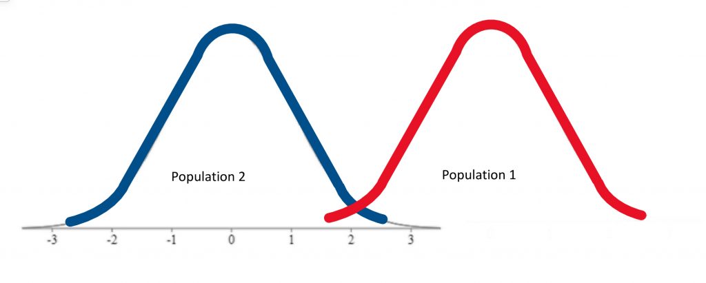
In other words, we were able to conclude that the difference between the centres of the two distributions was statistically significant.
If, on the other hand, the distributions were a bit less distinct, we would not have been able to make that claim of a significant difference.
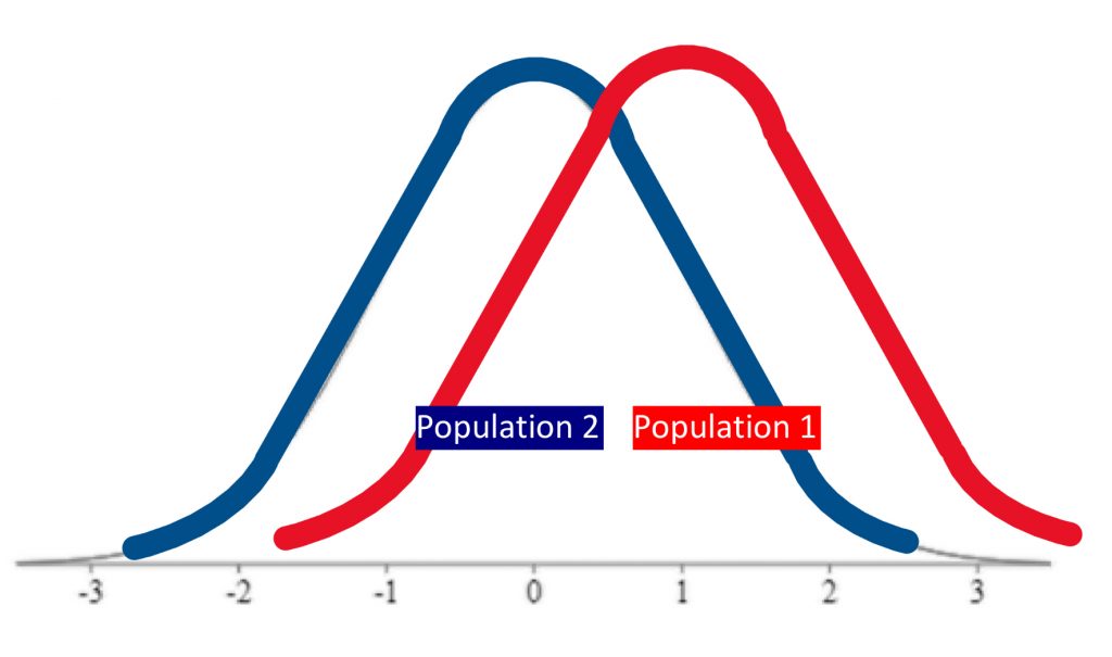
We would not have rejected the null hypothesis if evidence indicated the populations were too similar.
Just how different do the two distributions need to be? That criterion is set by the cutoff score, which depends on the significance level, and whether it is a one-tailed or two-tailed hypothesis test.
Concept Practice: Putting hypothesis test elements together
That was a lot of new concepts to take on! As a reward, assuming you enjoy memes, there are a plethora of statistics memes, some of which you may find funny now that you have made it into inferential statistics territory. Welcome to the exclusive club of people who have this rather peculiar sense of humour. Enjoy!
Chapter Summary
In this chapter we examined probability and how it can be used to make inferences about data in the framework of hypothesis testing. We now have a sense of how two populations can be compared and the difference between their means evaluated for statistical significance.
Key Terms:
| probability | research hypothesis | one-tailed test |
| central limit theorem | null hypothesis | non-directional hypothesis |
| population | cutoff sample score | statistical significance |
| sample | significance level | reject the null hypothesis |
| hypothesis testing | directional hypothesis | do not reject the null hypothesis |
Concept Practice
Return to text
Return to text
Return to text
Return to text
Return to text
Return to text
Return to text
Return to text
Return to text
Return to text
Return to text
Return to text
Return to text
Return to text
Return to 4a. Probability and Inferential Statistics
Try interactive Worksheet 4a or download Worksheet 4a
Return to 4b. Hypothesis Testing
Try interactive Worksheet 4b or download Worksheet 4b
video 4a2
video 4b2
in a situation where several different outcomes are possible, the probability of any specific outcome is a fraction or proportion of all possible outcomes
mathematical theorem that proposes the following: as long as we take a decent-sized sample, if we took many samples (10,000) of large enough size (30+) and took the mean each time, the distribution of those means will approach a normal distribution, even if the scores from each sample are not normally distributed
all possible individuals or scores about which we would ideally draw conclusions
a formal decision making procedure often used in inferential statistics
the individuals or scores about which we are actually drawing conclusions
the probability level that we are willing to accept as a risk that the score from our research sample might occur by random chance within the comparison distribution. By convention, it is set to one of three levels: 10%, 5%, or 1%.
critical value that serves as a decision criterion in hypothesis testing
prediction that the population from which the research sample came is different from the comparison population
the prediction that the population from which sample came is not different from the comparison population
a research prediction that the research population mean will be “greater than” or "less than" the comparison population mean
a hypothesis test in which there is only one cutoff sample score on either the lower or the upper end of the comparison distribution
a research prediction that the research population mean will be “different from" the comparison population mean, but allows for the possibility that the research population mean may be either greater than or less than the comparison population mean
a hypothesis test in which there are two cutoff sample scores, one on either end of the comparison distribution
a decision in hypothesis testing that concludes statistical significance because the sample score is more extreme than the cutoff score
the conclusion from a hypothesis test that probability of the observed result occurring randomly within the comparison distribution is less than the significance level
a decision in hypothesis testing that is inconclusive because the sample score is less extreme than the cutoff score
