2. Central Tendency and Variability
2a. Central Tendency
video lesson
In this chapter we will discuss the three options for measures of central tendency. These measures are all about describing, in one number, an entire dataset.
A measure of central tendency is a statistical measure that defines the centre of a distribution with a single score. The purpose of a central tendency statistic is to find a single number that is most typical of the entire group. It is a number that should represent the entire group as accurately as possible.
Depending on the shape of a distribution, one of these measures may be more accurate than the others. We will see that for symmetrical, unimodal datasets, the mean will be the best choice. For asymmetrical (skewed), unimodal datasets, the median is likely to be more accurate. For bimodal distributions, the only measure that can capture central tendency accurately is the mode.
It is very important to note that two out of three measures of central tendency only apply to numeric data. In order to arrive at a mean or a median, the data need to be measured in number form. It makes sense, for example, to measure the average student height in a class. It does not make sense to determine the average major from a class of students.
Before we can learn to calculate a mean, we need to familiarize ourselves with some statistical notation. In statistics, when we want to denote “taking the sum” of a series of numbers, we use the term Σ. This is the Greek capital letter S, known as “sigma”.
The tricky thing about Σ is learning how to use it within mathematical order of operations. You may remember the mnenonic BEDMAS from school. This indicates that you should first do any operations that are set off in brackets or parentheses. Next you should do exponents, then division or multiplication, and finally addition/subtraction. But summation fits in just after division/multiplication. So BEDMAS becomes BEDMSAS.
Order of Operations
BEDMSAS
| X |
| 5 |
| 8 |
| 9 |
| 6 |
| 7 |
![\[(\sum X)^{2}\]](https://pressbooks.bccampus.ca/statspsych/wp-content/ql-cache/quicklatex.com-a55c06814cae3ad9de01319b43b6f1b5_l3.png "Rendered by QuickLaTeX.com")
What is that telling you to do? Look at order of operations. First do anything in brackets. So first we have to do the ΣX part. This tells us to add up all the scores: 5+8+9+6+7 = 35. Next we need to take that result and square it (exponents): 352 = 1225.
Let us try:
![\[\sum X^{2}\]](https://pressbooks.bccampus.ca/statspsych/wp-content/ql-cache/quicklatex.com-e1d821e5c6bc3fd3fb7ca51c6b34c0d2_l3.png "Rendered by QuickLaTeX.com")
Now there are no brackets, so exponents come first. This formula says to square each score in the dataset, then add together all the results: 52+82+92+62+72 = 25+64+81+36+49 = 255. So what seems like a minor difference in the formula really changes the result!
Let us try:
![\[\sum (X-1)^{2}\]](https://pressbooks.bccampus.ca/statspsych/wp-content/ql-cache/quicklatex.com-f08c9467d2573984195010f41bf5dd36_l3.png "Rendered by QuickLaTeX.com")
First brackets, so subtract off 1 from each score. Next exponents, so square each result. And finally summation, so add that all together. 42+72+82+52+62 = 16+49+64+25+36 = 190.
And finally, we will try:
![\[\sum X-1^{2}\]](https://pressbooks.bccampus.ca/statspsych/wp-content/ql-cache/quicklatex.com-6f68780ab74e1dea857c98e79dde76f4_l3.png "Rendered by QuickLaTeX.com")
Now exponents is first, so square the number 1. Next is summation, so add all scores together. Finally, complete the subtraction. 12 = 1. 5+8+9+6+7 = 35. 35 – 1 = 34.
So, now you see that order of operations is vital to decode summation notation. Each of these variations have very different solutions. Whenever you see a new formula, try translating it into words after reviewing order of operations.
Now we are ready to take a look at calculating a mean. The mean is the most common measure of central tendency, because it has some powerful applications in statistics. The mean is the same thing as an average, something you are very familiar with. You also probably know that to find an average, you add up all the numbers, then divide by how many numbers there were.
![\[M=\frac{\sum X}{N}\]](https://pressbooks.bccampus.ca/statspsych/wp-content/ql-cache/quicklatex.com-55341b44493248a86727a0eed0aad993_l3.png "Rendered by QuickLaTeX.com")
In statistical notation, the formula for the mean is shown above. A mean is symbolized as M. The number of scores in a dataset is symbolized as N.
Conceptually we can think of the mean as the balancing point for the distribution. In a histogram, if we were to mentally convert the X-axis into a scale, the mean would be the fulcrum, or the point of the scale at which the two sides of the scale balance each other out. Each score is like a weight. Their position along the scale determines where the mean will be. Here are some examples.
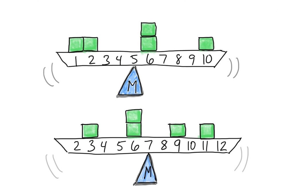
If we put it close to the middle of the scale, for example at 5, the scale would tip to the right. So we have to move the balance point rightward. Let’s see if that intuition is correct: M = (1+2+3+4+5+6+6+7+7+7+8+8+8+8+9+9)/16 = 6.1
The median, unlike the mean, is a counting-based measure. The values of the the scores are not important, just how many of them there are. To get the median, you find the midpoint of the scores after placing them in order. The median is the point at which half of the scores fall above and half of the scores fall below. Finding the median for an odd number of scores is easy. Just find the single middle score, and that is the median.
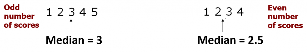
For an even number of scores, it is a little more complicated. You have to find the middle two scores and average those together.
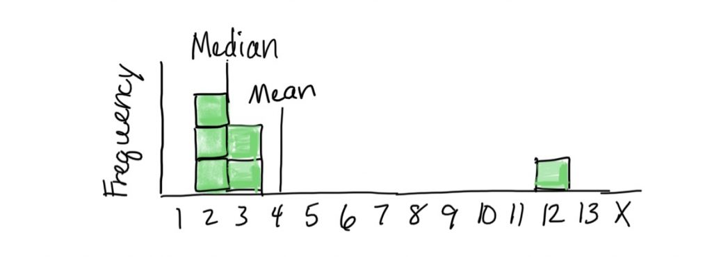
Here are some graphical examples of medians.
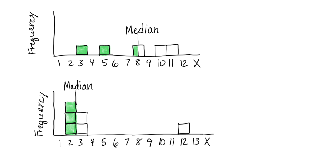
In the top histogram, 2 scores are below the median of 8, and two scores are above. Notice the median is not a balancing point (which would be a little to the left to account for the spread of the lower scores). In the bottom histogram, there are 2 scores below and two scores above the middle set of scores (2 and 3, averaged to 2.5). The median is not a balancing point (which would need to be further to the right to account for the score weighting down the right end of the scale).
The mode is our final option for statistical measures of central tendency. The mode is simply the score that occurs most often in the dataset, the one with the highest frequency. This is the measure that can be used with nominal data too. It is possible to have more than one mode, if the dataset is bimodal, for example. In fact the term unimodal means “one mode” and bimodal means “two modes”. Note that the mode must correspond to an actual score in the dataset, so a grouped frequency table or histogram will not help you identify it.
Another thing to note is that if your dataset happens to have two modes, that does not necessarily mean it is appropriate to describe the distribution as bimodal. Remember, true bimodal distributions are ones that show two distinct peaks in the smoothed line with some space between, indicating there are two collections of scores that are clustered together. Basically, if the distribution does not look like a camel’s back, then it is not truly bimodal.

2b. Variability
video lesson

In the image at left, it is easy to detect a difference in pattern among the rows — even though there are variations, there is also a clear theme. The butterflies on the top are dark with large light patches, and those on the bottom are light with dark trim. In the image at right, there is no clear theme in colouring pattern top to bottom, and there is a lot of variability in beetle appearance within each grouping. This is important, because if we want to be able to assert differences in what is typical or representative between one group and another, we need enough uniformity to discern those differences. If there is too much random variability, we will be unable to say much about the data or use them for decision making.
Our objectives in this part of the chapter will be that to explain the concept of variability and why it is important, and to calculate the descriptive statistics variance and standard deviation.
Soon we will be progressing to inferential statistics, in which we will often wish to figure out if the central tendency of one group of scores is different from another group of scores. If we want to be able to assert differences in what is typical between one group and another, we need enough uniformity within each of those groups to discern those differences. If there is too much random variability, we will be unable to say much about the data or use them for decision making. There will be too little order in the chaos. For that reason, we need to learn how to measure variability in a data set and take that into account in the process of making inferences about the data.
There are many ways to measure variability. However, we will focus on the two main measures of variability that are commonly use in both descriptive and inferential statistics of the sort we will cover in this course: variance and standard deviation. It is worth noting that variance and standard deviation are directly related, but standard deviation is easier to interpret and is thus more often reported as a descriptive statistic.
In general, measures of variability describe the degree to which scores in a data set are spread out or clustered together. They also give us a sense of the width of a distribution. Finally, they help us understand how well any individual statistic (for example the mean) can possibly represent the distribution as a whole.
When it comes to inferential statistics, smaller variability is better. When comparing two distributions, as we will be doing in inferential statistics, there are two ways to be confident that there is a difference. One is to have dramatically different central tendencies (such as the means). The other way is to have small variability, such that an individual statistic represents that distribution well.
The first measure of variability we will learn to calculate is variance. Variance summarizes the extent to which scores are spread out from the mean. To do that, we calculate the deviation of each score from the mean.
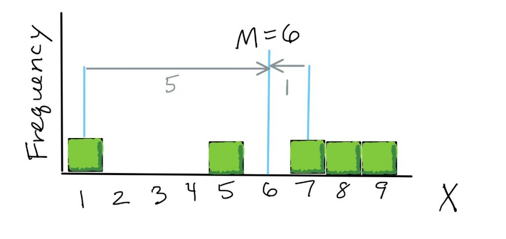
Here is a graphical illustration of deviations. As the first step in calculating variance, for each score we find its distance from the mean. So here if the distribution’s mean is 6, a score of 1 is a deviation of 5 away from the mean, and a score of 7 is a deviation of 1 away from the mean.
Here is the formula to calculate variance.
![\[SD^{2}=\frac{\sum (X-M)^{2}}{N}\]](https://pressbooks.bccampus.ca/statspsych/wp-content/ql-cache/quicklatex.com-1e00fac0117abd1c58db2dad8d0e5fb8_l3.png "Rendered by QuickLaTeX.com")
Steps to Calculate Variance
- Take the distance, or “deviation”, of each score from the mean
- Square each distance to get rid of the sign
- Add up all the squared deviations
- Divide by the number of scores
The first part of the formula we need to calculate, then, is to take the distance, or “deviation”, of each score from the mean. This is written as X-M.
Next, we square each distance to get rid of the sign (because some deviations will be negative numbers, which we do not want. This is the exponent outside the brackets.
Next, we do summation, so we add up all the squared deviations. In fact, the result of this step has its own name: Sum of Squares, which we will sometimes abbreviate as SS.
And finally, we divide by the number of scores, to make sure this is an average measure of distances in the dataset. Now, we’re doing the division last, because of the notation, because there is a top and a bottom. So that makes it clear that the division is the last thing that we do in the order of operations.
One thing to note is that the purpose of squaring each deviation before taking the sum is the following. All the deviations for scores smaller than the mean will come out negative. All the deviations for scores larger than the mean will come out positive. So if we added up the deviations without squaring them, the negatives would cancel out the positives and the variance would always end up zero. Squaring each deviation is mainly a way to convert them all to positive numbers.
Standard deviation is the other measure of variability we will use in this course. It expresses the variability in terms of a typical deviation in the data set. This will be a single number that gives us the distance of typical scores in the dataset from the mean.
Variance is essentially the average squared deviation; now we want to find the average deviation to get it back into the original units of the data. To find the standard deviation, we just need to take the square root of the variance.
![\[SD=\sqrt{SD^{2}}\]](https://pressbooks.bccampus.ca/statspsych/wp-content/ql-cache/quicklatex.com-691b36862848544bb4a135c64ec0d469_l3.png "Rendered by QuickLaTeX.com")
Most of the inferential statistics we will use in this course will be based on our calculations of the mean and either the variance or standard deviation.
Concept Practice: variability
Chapter Summary
In this chapter we examined the purpose and common methods for determining statistics representing the central tendency and the variability of a dataset. We saw the particular characteristics of each statistic that makes it most appropriate or useful for specific situations. The combination of central tendency and the variability statistics not only provides a very succinct summary of the dataset, but it also will become the basis for making inferences from data.
Key Terms:
| mean | Σ | variance |
| median | M | standard deviation |
| mode | N | Sum of Squares |
Concept Practice
Return to text
Return to text
Return to text
Return to text
Return to 2a. Central Tendency
Try interactive Worksheet 2a or download Worksheet 2a
Return to 2b. Variability
Try interactive Worksheet 2b or download Worksheet 2b
video 2a2
the same thing as an average: you add up all the numbers, then divide by how many numbers there were. Conceptually we can think of the mean as the balancing point for the distribution.
the midpoint of the scores after placing them in order. The median is a counting-based measure: the point at which half of the scores fall above and half of the scores fall below.
the score(s) that occur(s) most often in the dataset
in summation notation, a symbol that denotes “taking the sum” of a series of numbers
the symbol for the mean (average) of scores in a sample
the symbol for the number of scores in a sample
a common measure of variability in numeric data. The average squared distance of scores from the mean.
a common measure of variability in numeric data. The average distance of a scores from the mean.
the sum of squared deviations, or differences, between scores and the mean in a numeric dataset
