5. Single Sample Z-test and t-test
5a. Single Sample Z-test
video lesson
Now that you have mastered the basic process of hypothesis testing, you are ready for this: your first real statistical test. First, we will examine the types of error that can arise in the context of hypothesis testing.
Which type of error is more serious for a professional? 1. I decide that a new mode of transportation, the driverless car, is much safer than current modes of transportation, and recommend to the state that they force conversion to that new mode. But then it turns out after a year that the rates of accidents actually increased.

Or… 2. I decide that a new mode of transportation is safer than current modes, but I do not have enough confidence in that margin of safety and therefore do not recommend a sweeping change. After a year it becomes clear that driverless cars are indeed much safer, and a switch would have been beneficial.
If you selected the first error as the more serious one, then you chose a Type I error. This is the type of error that is considered more serious in the realm of statistical decision making, as well.
In the process of hypothesis testing, the decision you make is all about probabilities. It is an educated guess. However, there is always room for error. In fact, there are two types of errors you can make in hypothesis testing. Their imaginative labels are Type I and Type II error. As we saw, Type I error is considered more serious, so the Significance level is typically set with an eye toward the probability of Type I error that is deemed acceptable in that study. α = .05 indicates that the researcher accepts a 5% chance of a Type I error. In the decision matrix shown here, you can see how the hypothesis test can play out in four different ways.
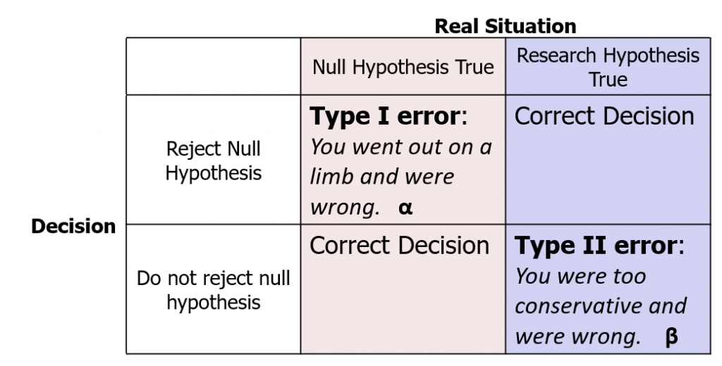
Note that the real situation, whether the null hypothesis is true or the research hypothesis is true, is unknown. We can never know which is true – that is why they are hypotheses, after all!
If, hypothetically, the null were true, and if we made the decision to reject the null hypothesis, then we would land in this corner of the decision matrix: Type I error. This is what happens if we go out on a limb, reject the null hypothesis, but we are wrong. As researchers we live in fear of making a Type I error. No one wants to make a big thing about their research findings and promote change to a new, different, risky, expensive thing, and then be wrong about it. On the other hand, if the null were true and we did not reject it, then we would be correct.
Hypothetically, let us suppose the research hypothesis were true. If we make the decision to reject the null hypothesis, then we are correct. However, if we decide not to reject the null hypothesis, we would be making a Type II error. This is when we are too conservative, decide there is not enough evidence that the research (alternative) hypothesis could be correct, but we are wrong. Type II error is also not great, so we do try to minimize that probability by doing something called a power analysis. However, researchers generally would rather make a Type II than a Type I error. Keeping the status quo may not do much for to make your scientific career exciting, but objectively speaking it is not such a scary proposition.
Now, a key thing to remember when you refer back to this decision matrix to determine for which error you are at risk, you never know which column you are in, because the real situation is always unknown. What determines the possible type of error is the thing you have control over: the decision. So you can switch the row you will place yourself in, depending on the observed data, and thus remove yourself from unreasonable risk of Type I error. (The probability of making a Type I error is symbolized as α, so significance levels are often referred to as α .)
Concept Practice: Type I and Type II errors
Okay, we are about to make a connection that is intellectually a bit challenging. So prepare yourself: we will be drawing connections between the central limit theorem, sampling distributions, and the appropriate type of comparison distribution we should use for a hypothesis test where the sample is made up of more than one data point.
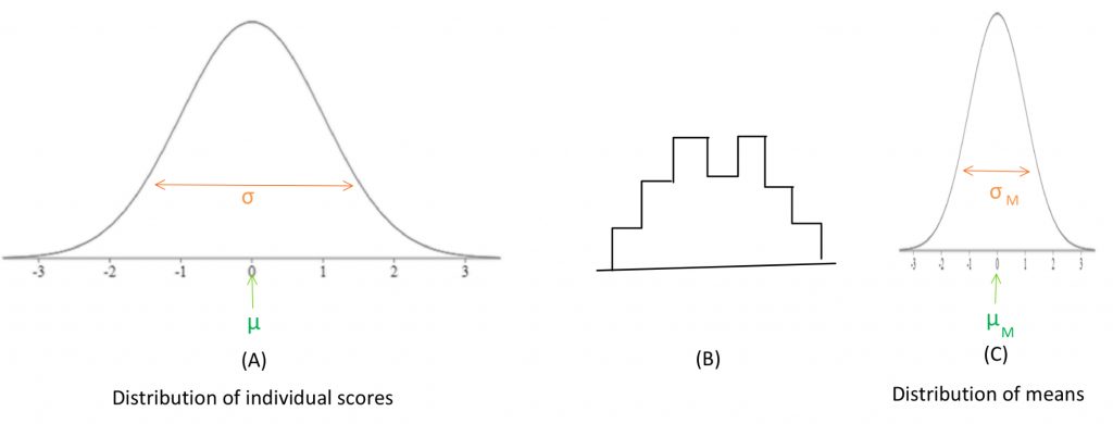
In the past, we have been using the normal distribution made of up individual scores as our comparison distribution. In the illustration below, if distribution (A) is the distribution of individual scores, (B) is the histogram of a sample of scores drawn from (A). (C) is the distribution of means from many samples such as the one portrayed in (B).
![\[\sigma^{2}_{M} = \frac{\sigma ^{2}}{N}\]](https://pressbooks.bccampus.ca/statspsych/wp-content/ql-cache/quicklatex.com-dddc6771e8e0567c6019f9e5447841fe_l3.png "Rendered by QuickLaTeX.com")
![\[\sigma_{M} = \frac{\sigma }{\sqrt{N}}\]](https://pressbooks.bccampus.ca/statspsych/wp-content/ql-cache/quicklatex.com-79feb6b9641740458aca68473e845118_l3.png "Rendered by QuickLaTeX.com")
![\[\mu_{M} = \mu\]](https://pressbooks.bccampus.ca/statspsych/wp-content/ql-cache/quicklatex.com-fc0b6112a05ecfa074076c4065a6129f_l3.png "Rendered by QuickLaTeX.com")
Concept Practice: Distribution of Sample Means
Up until now we worked with individuals as our samples, so we could use our old Z-score formula and compare the sample score to a comparison distribution of individuals. We did this, so that we could avoid adding new symbols to our formulas, and concentrate on the hypothesis testing logic. Now, we want the more realistic situation, so we will use the Z-test to compare a sample mean to a comparison distribution of sample means. To rephrase, when we had an individual score, we used the distribution of individuals. When we have a sample mean, we need to use the distribution of sample means. The new Z-test statistic formula is shown here:
![\[Z=\frac{M-\mu _{M}}{\sigma _{M}}\]](https://pressbooks.bccampus.ca/statspsych/wp-content/ql-cache/quicklatex.com-441e8a64eccfe6c4e748fb4c2a49b5f0_l3.png "Rendered by QuickLaTeX.com")
In this formula, M is the sample mean, μM is the comparison distribution mean, and σM is the comparison distribution standard deviation.
We will be using the terminology “distribution of means,” because it’s a name that reminds us of how it differs from the distribution of individuals. A term in statistics that means the same thing is “sampling distribution.” Why do we need this distribution of means? In reality, we do not compare an individual sample score against a population distribution of individuals. For a real statistical test, we collect a sample and calculate a mean, and compare that sample mean against a comparison distribution of means. We will ground that in an example: If I want to know if my introductory psychology class is collectively performing at the expected level on a test, I do not take their average performance and compare that mean against a set of individual scores, I want to compare it to a set of other class averages. How does this impact our hypothesis test? It matters for Step 2, determining the characteristics of the comparison distribution. Well, it does not change anything about the comparison mean, because the mean of a distribution of means is equal to the mean of the distribution of individuals. But the standard deviation now needs to be converted into the standard deviation of the distribution of means, which is often called the standard error of the mean. As these equations above show, the variance of a distribution of means is equal to the variance of the distribution of individuals divided by the number of individuals in the sample. And thus, if we take the square root of the variance, the standard deviation of a distribution of means is equal to the standard deviation of the distribution of individuals divided by the square root of the number of individuals in the sample.
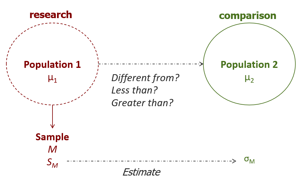
We will now examine the way the steps of the hypothesis test procedure play out when using the single-sample Z-test. First, we need to formulate the research and null hypotheses. Remember, in such a hypothesis test, we are trying to compare two populations. Population 1, the research population, is the one from which we have drawn a research sample.
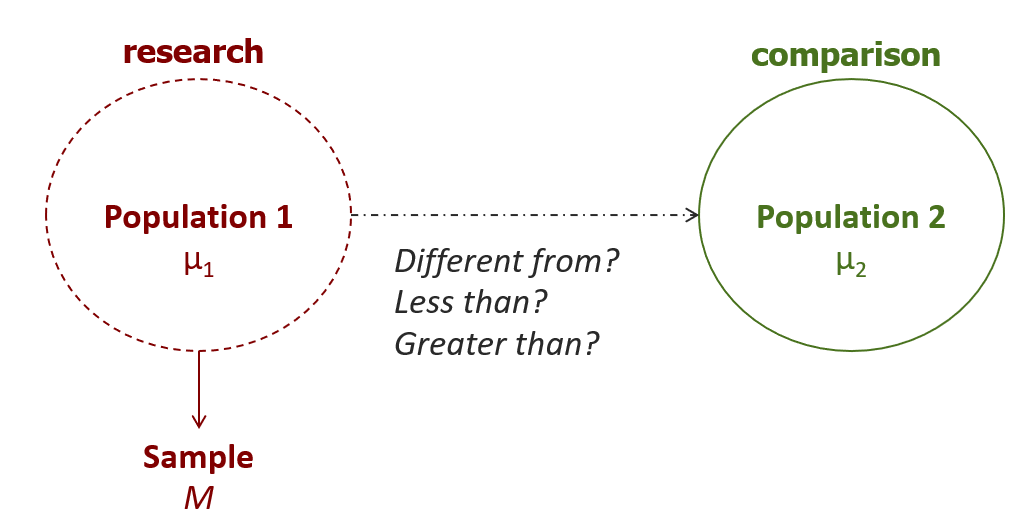
We do not have access to the actual research population mean, hence the need to calculate a sample mean. That sample mean is our best proxy for the population 1 mean, which we need to compare to the mean of population 2. The nature of the comparison, in particular its directionality, is determined by the researcher’s prediction.
In step 2, we need to determine the characteristics of the comparison distribution. This means that we need the mean and standard deviation of the comparison distribution, which represents Population 2. This is where we need to introduce the new distribution of means. The mean is the same as provided, but the standard deviation needs to be converted.
If the variance is provided, you can start with this formula to convert to the distribution of means, then take the square root to get the standard deviation:
If the standard deviation is provided, it is easiest to use this formula:
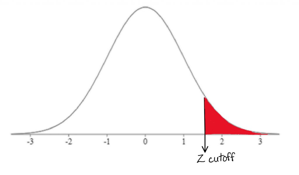
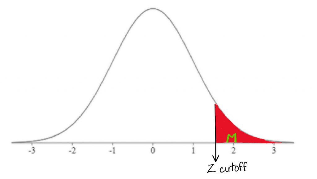
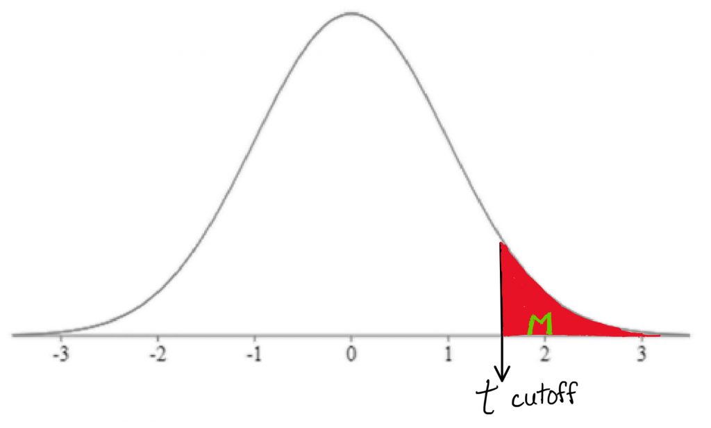
Step 3 is to determine the cutoff sample score, which is derived from two pieces of information. First, we need to know the conventional significance level that applies. Second, we need to know which tail we are looking at. The bottom, the top, or both? This depends on the research hypothesis, so we should always look for directional keywords in problem. If the research hypothesis is directional, we should use a one-tailed test. If the research hypothesis is non-directional, we should use a two-tailed test.
Once we have those two pieces of information, we can find the Z-score that forms the border of the shaded tail by looking it up in a table. We can then map the cutoff score onto a drawing of the comparison distribution.
In step 4, we need to calculate the Z-test score from the sample mean:
In this formula, M represent the research sample mean, μM represents the comparison population mean, and σM represents the standard deviation of the comparison population. Remember, we are using the distribution of means as our comparison distribution. Once we have calculated the Z-test score, we will mark where it falls on the comparison distribution, and determine whether it falls in the shaded tail or not.
Finally, it is time to decide whether or not to reject the null hypothesis. If the sample mean falls within the shaded tail, we reject the null hypothesis. If it does not, we do not reject the null hypothesis. In other words if the sample mean is extreme enough relative to the comparison distribution of means, then we reject the null hypothesis.
Once we make our decision, we will need to take a close look at what kind of error we might have made as a result of our decision. And remember, from our decision matrix, all we have control over whether we’re on the top row or the bottom row.
We do not know the real situation. if we do make the conclusion that we should reject the null hypothesis, then we are at some risk of a Type I error, but as long as we don’t exceed our significance level, we accept that risk. If we do not reject the null hypothesis we could be at a risk for Type II error.
Typically, after conducting a hypothesis test, researchers want to obtain the p-value, or the probability of the observed sample score or more extreme occurring just by random chance under the comparison distribution. The p-value associated with the sample mean has to be less than the significance level in order to reject the null hypothesis. A common way to find the p-value is to use an online calculator.
One last exercise I would like you to try is to pretend you are publishing these results in a scientific journal. So you might write this sentence in your results section based on your findings: “We found that patients with insomnia who received a new drug slept significantly more than patients who did not receive the new drug (p < .05).”
Notice the term “significantly” is used in this example, because the null hypothesis was rejected at the end of the hypothesis test. Also, the p-value is in brackets at the end of this sentence, before the punctuation, just like you would use a citation to back up a factual claim… only here, it is a claim of statistical significance.
Concept Practice: Conducting a Z test
5b. Single-sample T-test
video lesson
Now it is time to introduce your second real statistical test: the single-sample t-test. This test is much like the Z-test, but more commonly used in real life.
Before we get started on the t-test, I am curious… would you have greater confidence in a statistic that comes from a small sample?

Or in one that comes from an entire population?… If you said that you would have greater confidence in a number that comes from an entire population, then the field of statistics would agree with you.
Sometimes, though, we do not have access to all the data from population that we need, and we have to take a best guess based on a sample. In that case, we probably want to be more conservative in our decision making. That’s what a t-test is for.
Often, even if we have information regarding the comparison population mean, we do not have access to the population standard deviation (σ). In this situation, what we must do is collect a sample reflecting population 1, calculate its mean and standard deviation, and compare that sample mean against a comparison distribution of means using an estimate (SM) of the population (σM). Note the change in symbol (from σ to S) to reflect the fact that we are basing our estimate on sample data, rather than using a known population parameter.
![\[S^{2} = \frac{\sum (X-M)^{2}}{N-1}\]](https://pressbooks.bccampus.ca/statspsych/wp-content/ql-cache/quicklatex.com-de768ae958fbd82bbc987d55b4a263fb_l3.png "Rendered by QuickLaTeX.com")
You may have noticed that this new formula for calculating variance in a sample has on the bottom “N minus 1” rather than just “N” as our old calculation formula had. Why “N minus 1”? This is a correction, based on sample size, that derives from the concept of degrees of freedom. We will return to that concept later. For now, let us consider “N minus 1” as a correction based on sample size that has the following deliberate and intentional effects on our calculation. If we have a small sample size, in which we should not have a great deal of confidence, subtracting 1 really affects the calculation. For example, if we had an N of 2, subtracting off 1 from that sample size will mean that we divide by 1 instead of 2. That has a drastic impact on the variance calculation, in effect doubling our estimated variance. Of course in the context of hypothesis testing, more variance is bad – in that we are less likely to be able to make conclusions based on the data.
On the other hand, with a larger sample size, subtracting 1 will have little impact on our calculation… dividing by 100 or dividing by 99 will have nearly identical results. Think of it this way – if we have a small sample size, we are punishing ourselves, like a handicap in a golf game. With a larger sample size, we reward ourselves, boosting our chance of a conclusion statistical decision.
Subtracting off 1 is like a flat tax – a flat income tax of 10% for all Canadians would be harder on those with a low income, who would have even less money to meet basic survival needs, whereas the wealthiest Canadians would still have plenty of money for their needs. That is, of course, why democratic governments typically use progressive tax rates, because those who have more can afford to pay a greater proportion of their income and still have enough to cover their basic costs of living. With hypothesis testing, though, the flat tax is desirable, because it is our intent to penalize the smallest sample sizes the most, given the fact that we can have little confidence in the estimates we derive from them.
The t-test is designed around the concept of degrees of freedom, which is defined as the number of scores in a given calculation that are free to vary. This is an abstract definition that is difficult to grasp, so it is helpful to consider a concrete example.
Degrees of Freedom Practical Example
First, consider the game of baseball. We understand the field-of-play consists of 9 positions. The coach is “free” to assign any of the 9 players to any of the 9 positions. Once the 8th player is assigned to the 8th position, the 9th player-position is pre-determined, so to speak. In other words, the coach is not “free” to pick either the last position or the last player.
Source: https://www.isixsigma.com/ask-dr-mikel-harry/ask-tools-techniques/can-you-explain-degrees-freedom-and-provide-example/
The same logic holds when doing a calculation involving all of a sample’s scores. Up until the last score inputted into the formula, the scores are free to vary; but the last score is pre-determined. Thus degrees of freedom in a t-test is N-1, or 1 less than the total number of scores in the dataset.
In a t-test we will be using the t-distributions, rather than a normal distribution, as our comparison distributions. The t-distributions are a series of distributions, based on the normal distribution, that adjust their shape according to degrees of freedom (which in turn is based on sample size).
As mentioned previously, when we do not have the population standard deviation we must estimate it from our sample. This involves a greater risk of error. The risk is related to how large our sample is. So, the fewer the scores in our sample, the fewer the degrees of freedom, and the more conservative the distribution we must use – one that is wider and shorter (more area in the tails).
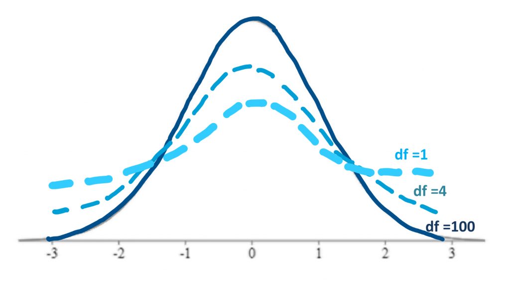
Above you can see examples of how the shape of the t-distributions changes with reduced degrees of freedom. With degrees of freedom of 100, the shape of the distribution is very close to the normal curve. If we have very few degrees of freedom, like 1, then our shading rejection regions, or goal posts, will move farther out into the tails of the distribution, because there is more area under the tails of the curve. In effect, then, with fewer degrees of freedom, we will find it more difficult to reject the null hypothesis. This is, of course, by design, in order to penalize the hypothesis test if it is based on a very small sample size.
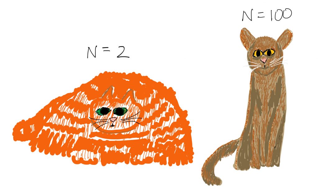
Above is a less technical visual to see the difference in distribution shape when the sample size is small, versus when the sample size is large. As you can see, when you have a large sample size, the goal posts are very close and easy to reach, but when you have a small sample size, they will really be far away, and this will make it difficult to reject our null hypothesis.
Concept Practice: Sample size and the t-test
Now we are ready to take a look at how a hypothesis test works based on a single-sample t-test. As before, the structure of the test is familiar – we are comparing the means of Population 1 and Population 2.
As usual, we do not have access to the mean of population 1, just the mean of a sample from that population. Furthermore, unlike in a Z-test, we do not have access to one piece of information about population 2: the population standard deviation. Therefore, we will form hypotheses the same way, but when we do steps 2 and 4, we will need to use the sample to generate an estimate of the comparison population standard deviation.
Concept Practice: When to use a Z-test or a t-test
In step 2, we identify the known comparison population’s mean. However, we will need to use the sample to generate an estimate of the comparison population standard deviation. We calculate the sample variance, using the formula with the “N-1” correction,
and then convert the variance to the distribution of means by dividing by N,
![\[S^{2}_{M} = \frac{S ^{2}}{N}\]](https://pressbooks.bccampus.ca/statspsych/wp-content/ql-cache/quicklatex.com-6635a18895337a42d755b86265f91da3_l3.png "Rendered by QuickLaTeX.com")
and finally we square root to get from variance to standard deviation.
![\[S_{M} = \sqrt{S^{2}_{M}}\]](https://pressbooks.bccampus.ca/statspsych/wp-content/ql-cache/quicklatex.com-68bfd289ef9453b6d47c1db3733eca96_l3.png "Rendered by QuickLaTeX.com")
SM is what we will use to describe our comparison distribution.
In step 3, as before we need to find our cutoff sample score based on the significance level and directionality of the test. Now, however, we also need to use a third piece of information: degrees of freedom. This is found by subtracting one from the sample size. Then we can look in the t-tables, identifying the row of the table with the matching degrees of freedom, then looking in the appropriate column based on directionality and significance level. Once we identify the t-score that forms the border of the shaded tail, we can map this onto a drawing of the comparison distribution. For visualization purposes, it is fine to sketch the distribution the same way you did the normal distribution.
Concept Practice: Degrees of Freedom
Now for step 4. The t-test formula is just like the Z-test one on top – sample mean minus comparison population mean. Then you divide by SM, the estimate of standard deviation that you calculated back in step 2.
![\[t = \frac{M-\mu _{M}}{S_{M}}\]](https://pressbooks.bccampus.ca/statspsych/wp-content/ql-cache/quicklatex.com-30bb6392ec2914d450cd79778fcd7ad1_l3.png "Rendered by QuickLaTeX.com")
If your calculated t-test score fell into the shaded tail beyond your cutoff score, then you may reject the null hypothesis. In other words, if the sample mean was extreme enough on the comparison distribution of means, reject the null.
After conducting a hypothesis test, it is helpful to also obtain a report the precise p-value associated with the result. The p-value offers the precise probability of obtaining the t-test result (or more extreme) just by random chance under the comparison distribution. It is found by calculating the area under the comparison distribution in the tail beyond the observed t-test score calculated in step 4 (or in both tails, if it was a two-tailed test).
Concept Practice: Conduct a t-test
Concept Practice: Facts about Z- and t-tests
Chapter Summary
In this chapter we learned about the two types of logical errors we can make in hypothesis testing: Type I and Type II errors. We saw that Type I error is considered more serious in statistics, because it represents going out on limb, making a strong conclusion, when that is in fact the wrong decision. For that reason, Type I error risk is strictly controlled in inferential statistics by setting a particular significance level (α). We also introduced our first real inferential statistical tests: the single-sample Z-test and the single-sample t-test. In each of these tests, we are comparing the means of two populations, using a sample to estimate the mean of the research population. A Z-test is used when we know the standard deviation of the comparison population (σ); a t-test is used when we do not have that information and must estimate the standard deviation from the sample (S).
Key terms:
| Type I error | distribution of means | p-value |
| Type II error | Z-test | t-test |
| α | standard error of the mean | degrees of freedom |
Concept Practice
Return to text
Return to text
Return to text
Return to text
Return to text
Return to text
Return to text
Return to text
Return to 5a. Single-sample Z test
Try interactive Worksheet 5a or download Worksheet 5a
Return to 5b. Single-sample t test
Try interactive Worksheet 5b or download Worksheet 5b
video 5a2
if we made the decision to reject the null hypothesis when it is true
if we made the decision to not reject the null hypothesis but the research hypothesis is true
the probability of making a Type I error; used as shorthand for significance level
also called a sampling distribution, is the distribution of many sample means drawn from the population of individual scores
statistical hypothesis test suitable for comparing the means of two populations, when the comparison population mean and standard deviation are known
standard deviation of the distribution of means
the probability of the observed sample score or more extreme occurring at random under the comparison distribution
statistical test to test the differences between two population means. Suitable for single sample design when standard deviation is unknown, or in two-sample designs.
the number of scores in a given calculation that are free to vary.
