7. Independent Means t-test
7. Independent Means t-test
In this chapter, I will introduce to you one last t-test variation – the independent means t-test. This one is intended for the classic experimental design, in which two independent samples are compared.

In a classic experimental design, we are comparing two samples. The independent means t-test is typically used to compare the data from an experimental group to those from a control group. The experimental group is the one that receives the manipulation, or the independent variable, and the control group is the one that receives either no manipulation, or an alternative one that represents the status quo – like a placebo. What makes this different from the repeated measures type of design, is that the scores from the two groups are independent. They are obtained from different participants who are randomly assigned to one group or the other.
For example, if I want to see if memory span is affected by the colour in which items are presented. I test one group of people with black and white items, and test another group of people with red items.
I will compare one group average with the other group average. There is no relationship or dependency of one group of scores with the other group, so it will be appropriate to analyze the data with an independent t-test.
With all statistical tests, we know each sample comes from a population. The question is: are they different populations? To answer this question using statistical tests, we need to make some assumptions about the data. We have been making the normal curve assumption all along, and we saw how the central limit theorem can be used to justify this assumption when our samples are large enough. With this new kind of t-test, we are also going to make the homoscedasticity assumption: that the two populations we are comparing have the same variance. In an introductory course like this, we will not go into the technicalities of verifying this assumption, but it is possible to do so before we conduct the analysis.
In the independent means t-test, just like with the dependent t-test, we have no direct information about population 1 or 2. We calculate sample means from our research and comparison samples. To find the standard deviation for the comparison population, we will take sample based estimates using all the scores we have to hand, by pooling together the variance of each sample. This makes sense if we are assuming the two populations have equal variance.
In step 2, we will once again set the comparison population mean to zero, because the comparison reflects the distribution of means under the null hypothesis, in which there is no difference between the populations.
![]()
The standard deviation will be calculated through a workflow previous students have told me looks like an hourglass shape.
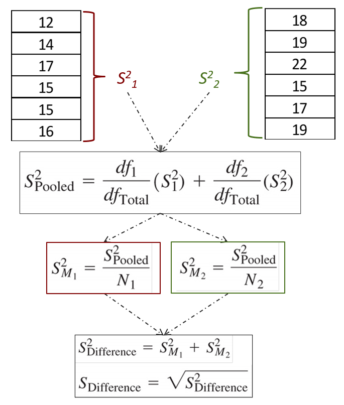
Starting from the top, we first calculate the variance of sample 1 and sample 2 separately.
![\[S^{2}=\frac{(X-M)^{2}}{N-1}\]](https://pressbooks.bccampus.ca/statspsych/wp-content/ql-cache/quicklatex.com-cda4a90a7d273c0103b22ca99d0a5165_l3.png "Rendered by QuickLaTeX.com")
We then pool the two variances together using a weighted average formula. This formula just allows us to count one variance more than the other if the sample size is bigger. With two independent samples, it is not uncommon to have an unequal N, or number of scores, in each group.
![\[S^{2}_{Pooled}=\frac{df_{1}}{df_{Total}}(S^2_{1})+\frac{df_{2}}{df_{Total}}(S^2_{2})\]](https://pressbooks.bccampus.ca/statspsych/wp-content/ql-cache/quicklatex.com-104123388f6a77e74f68ec9c28d1a5f0_l3.png "Rendered by QuickLaTeX.com")
Once we have the pooled variance calculated, we use that to convert to the variance of the distribution of the difference between means, which is the comparison distribution for this test.
![\[S^{2}_{M}=\frac{S^{2}_{Pooled}}{N} \]](https://pressbooks.bccampus.ca/statspsych/wp-content/ql-cache/quicklatex.com-a3862cc74a7196cf8599278e700f391f_l3.png "Rendered by QuickLaTeX.com")
![\[S^{2}_{Difference}=S^{2}_{M1}+S^{2}_{M2} \]](https://pressbooks.bccampus.ca/statspsych/wp-content/ql-cache/quicklatex.com-8a697044b808b6a937f9e9907ef65c24_l3.png "Rendered by QuickLaTeX.com")
We then square root to get the estimated standard deviation for the comparison distribution.
![\[S_{Difference}=\sqrt{S^{2}_{Difference}} \]](https://pressbooks.bccampus.ca/statspsych/wp-content/ql-cache/quicklatex.com-899537b8a778791340ee3725c9b28c16_l3.png "Rendered by QuickLaTeX.com")
Now for step 3: the one new thing here is the degrees of freedom we will use to look up the cutoff sample score in the t tables. Because we have two samples, we will use the pooled, or total, degrees of freedom for lookup. That is the main advantage of the independent means t-test. Because we have two samples of scores, we get the benefit of more degrees of freedom.
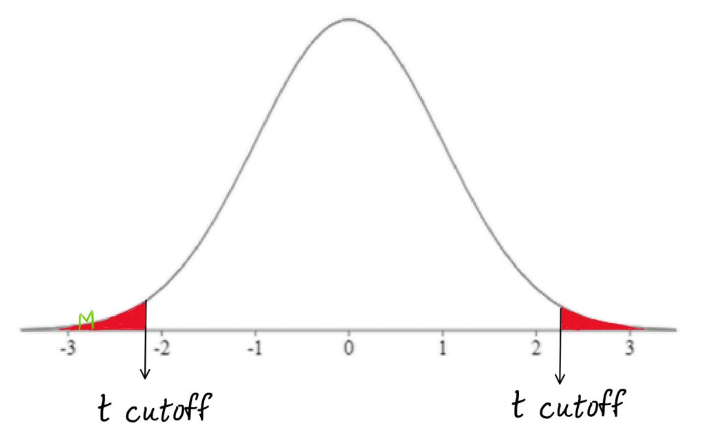
For step 4, we have a new t-test formula. We subtract the sample mean of the control group from the sample mean of the experimental group, so that our directionality makes sense when we mark the test score on the comparison distribution and determine whether it falls in the shaded tail.
![\[t=\frac{M_{1}-M_{2}}{S_{Difference}}\]](https://pressbooks.bccampus.ca/statspsych/wp-content/ql-cache/quicklatex.com-104d8a5c6ca82a7fda7bd4f33a0af9de_l3.png "Rendered by QuickLaTeX.com")
One thing never changes: In step 5, if the t-test score falls in the shaded tail we reject the null hypothesis.
As we go through the course, we are repeating lots of concepts and procedure enough, that I start to go quickly through those elements. If some aspect of the hypothesis test is still not making sense, that’s totally okay, and it’s completely normal. But you need to come back to those bits and grapple with them, perhaps by heading back to earlier chapters where those concepts or procedures were first introduced. Do not give up on a concept if it is still fuzzy. By now things should be starting to gel. Are there any aspects that you are still doing by rote rather than through conceptual understanding? I recommend that you persist. It will make sense if you get enough examples and explanations. For most of us it takes quite a bit of repetition and a few different approaches. Check out another textbook for an alternative look at the same piece.
If we were writing up the hypothesis test outcome from the example illustrated above, we might interpret it this way in the results section: “We found that people who consumed chocolate had significantly lower mood scores than the control group (p = 0.0145).”
The p-value represents the probability of the test score, or any score that is more extreme than that, occurring under the comparison distribution. To get that, we find the area under the curve beyond the test score, either in one tail or in both tails, depending on the directionality of the test.
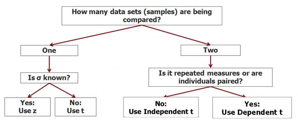
We have now completed the decision tree for this section of the course. If we have two samples to compare, and there is no relationship between the individuals in the two samples, we use the independent t-test.
Chapter Summary
In this chapter, we introduced the use of the independent means t-test in the context of hypothesis tests of the difference of two sample means. This test is appropriate for research designs in which two samples are formed through random assignment to groups, for example and experimental group and a control group. Scores from both samples are used to estimate the comparison population distribution, and to contribute to degrees of freedom.
Key terms:
| independent means t-test | normal curve assumption | homoscedasticity assumption |
a statistical test used in hypothesis tests comparing the means of two independent samples, created by random assignment of individuals to experimental and control groups
parametric tests like the t-test and Z-test require the assumption that the distribution of means for any given population is normally distributed
independent means t-tests require the assumption that the two populations we are comparing have the same variance
