6. Dependent t-test
6. Dependent t-test
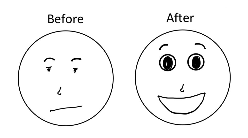
This chapter will introduce you to the dependent means t-test, which is most often used for experiments with a repeated measures design. Repeated measures designs are very common experimental approaches, just as posts on social media often compare before and after images to show off the effects of a diet or a renovation.
Repeated measures experimental designs are also known as within-subjects designs. Such an experiment involves obtaining two separate scores for each individual in the sample. Instead of having an experimental group and control group, there is just one sample, from which the same participants are used in all treatment conditions. Typically this kind of study uses a pre-test post-test design.
As an example, perhaps I want to see if memory span is affected by the colour in which items are presented. I first test people on black and white items, then test them with red items. I will compare their performance on the second test with their performance on the first test.
Another less-common type of experimental design that would be analyzed using a dependent t-test is the matched pairs design. In this type of approach, two separate samples are used, but each individual in a sample is matched one-to-one with an individual in the other sample. This is most commonly used when the researcher is intent on controlling for a possible confounding variable and thus matches participants based on that variable – for example, age or genetic relatedness. Because of this matching, the two samples are not independent, but rather they are related in some way. Hence the name “dependent t-test”.
This may not be a familiar idea, so we will consider an example of a matched pairs design. Perhaps I want to test differences in memory capacity in an experimental group and compare to a control group, but I know age can greatly impact this type of memory. So, I make sure for each person aged 20 in one group there is another person with the same age in the other group, and so on, for each age. That way, I am getting the difference in memory scores for each matched pair, and thus age is explicitly controlled for as a possible third variable.
As before, the first step of the hypothesis test is to formulate hypotheses. The goal is to compare the means of two populations. This time, though, we not only have no standard deviation from population 2, we also have no mean. For both populations, we will rely on sample-based estimates for the mean and the standard deviation. In a repeated measures experiment, we would have one set of scores measured at baseline, the before scores. These scores will represent population 2, the comparison population. The scores that are measured after the experimental manipulation will represent the research population, population 1.
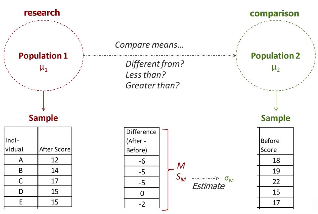
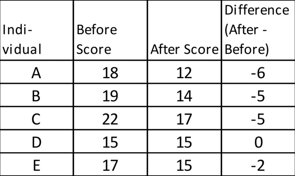
To conduct the comparison, we will actually take the difference score for each individual in the study, by subtracting the before score from the after score, and then calculate the mean and standard deviation of the difference scores. As an example, I made up some scores on a mood measure for people after eating chocolate and before eating chocolate, and calculated after-before difference scores for each individual (shown above). Negative difference scores indicate mood scores went down after eating chocolate; positive difference scores indicate mood scores went up after eating chocolate. (Worry not, this is a completely invented dataset — it seems unlikely to me that eating chocolate would actually worsen most people’s mood!)
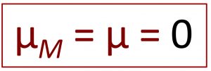
In step 2, we need to approach the mean and standard deviation of the comparison distribution a little differently than before. The comparison distribution will now be the distribution of means for the population of difference scores, which are defined as after-minus-before scores. Under the comparison population, the mean of difference scores should be 0: under the null hypothesis, there is no no difference between those who ate chocolate and those who did not, for example, so there would be no change before to after. Thus we set the mean of the comparison population to 0.
Now for the standard deviation: we will need to use the sample of difference scores to generate an estimate of the comparison population standard deviation. Perhaps you are wondering why we calculate difference scores as after-minus-before? This is important for the way we interpret the difference scores, and to fit the directionality of our hypothesis test. In our example, if people’s mood scores worsen, this should result in a negative difference score, moving the mean toward the low end of the distribution, right? And if the mood improves that should result in a positive score. That is why we have to set up the difference scores as after-minus-before.
If we look at these example data, right away by looking at the difference scores, we can tell the mood went down for almost every one, except for one person who did not change.
The formulas to calculate a sample-based estimate of the comparison distribution standard deviation are exactly the same as for a single sample t-test:
![\[S^{2}=\frac{(X-M)^{2}}{N-1}\]](https://pressbooks.bccampus.ca/statspsych/wp-content/ql-cache/quicklatex.com-cda4a90a7d273c0103b22ca99d0a5165_l3.png "Rendered by QuickLaTeX.com")
![\[S^{2}_{M}=\frac{S^{2}}{N}\]](https://pressbooks.bccampus.ca/statspsych/wp-content/ql-cache/quicklatex.com-886fa7d0dbe28fb653ca09fe970f1496_l3.png "Rendered by QuickLaTeX.com")
![\[S_{M}=\sqrt{S^{2}_{M}}\]](https://pressbooks.bccampus.ca/statspsych/wp-content/ql-cache/quicklatex.com-c3a85e3997046d8c7eda9bf8f6130b4e_l3.png "Rendered by QuickLaTeX.com")
In fact, that is why I wanted to introduce you to the dependent t-test before we move on to the independent t-test, which has a different set of formulas.
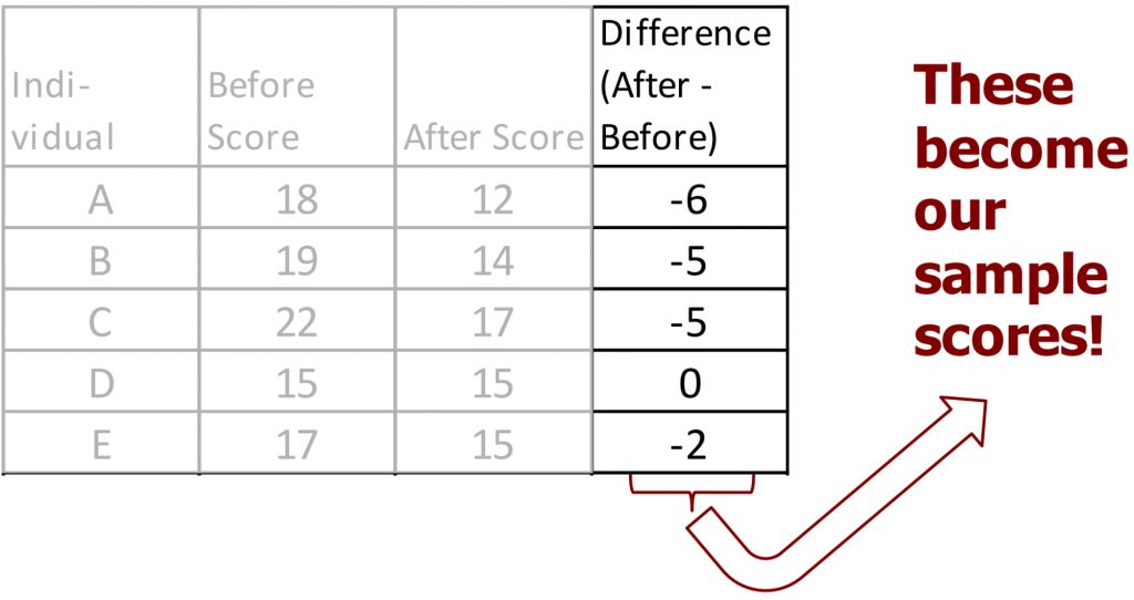
Before we get to our example, I would like to note that once we calculate the difference scores for each individual in the sample, we will be using those difference scores to calculate the mean and standard deviation. We no longer need the before or after scores for anything. I recommend crossing them out, so you are not confused about which numbers to include as X in the formulas.
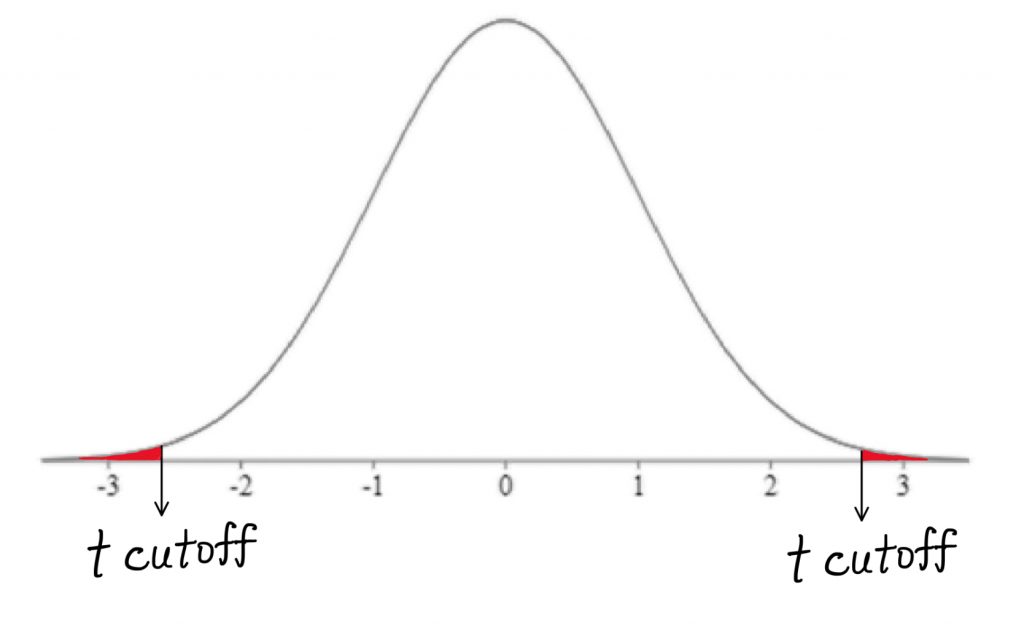
In step 3, we need to determine the cutoff sample score. As with the single sample t-test, this will be derived from three pieces of information: the significance level, the directionality, and degrees of freedom. We can use t-tables to find the cutoff score and map it onto our drawing of the comparison distribution.
Step 4 is the moment of truth – does the sample mean fall far enough from the comparison population mean to reject the null hypothesis? We can use the same t-test formula as for the single-sample t-test.
![\[t=\frac{M-\mu _{M}}{S_{M}}\]](https://pressbooks.bccampus.ca/statspsych/wp-content/ql-cache/quicklatex.com-f685bc696d4b21513d8d912cbcc50d9e_l3.png "Rendered by QuickLaTeX.com")
Remember, the comparison population mean is now set to zero, so we can use that in place of μ.
![\[t=\frac{M-0}{S_{M}}\]](https://pressbooks.bccampus.ca/statspsych/wp-content/ql-cache/quicklatex.com-3253d982efadf99d2838a80174852189_l3.png "Rendered by QuickLaTeX.com")
Once we have calculated the t-test result, we can mark it on comparison distribution to determine whether it falls in shaded tail or not.
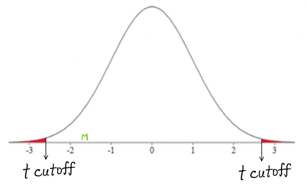
Finally, it’s decision time. Did the sample mean of difference scores fall within a shaded tail on the comparison distribution? Is it extreme enough to reject the null?
As always, we can also use a calculator find the p-value, the precise probability that this t-test score (or more extreme) would have occurred by random chance alone under the comparison distribution.
If you were writing these results for publication, how would you translate the hypothesis test into a concise sentence? Does the chocolate make people’s mood change? In this example, we found that mood scores were not significantly different after people consumed chocolate.
We can support that statement with the information that the probability of the sample mean occurring on the comparison distribution was more than 5%. As a result we have an inconclusive hypothesis test.
As we continue to build our decision tree, you can use it to guide your choice of a statistical test appropriate for a particular research design.
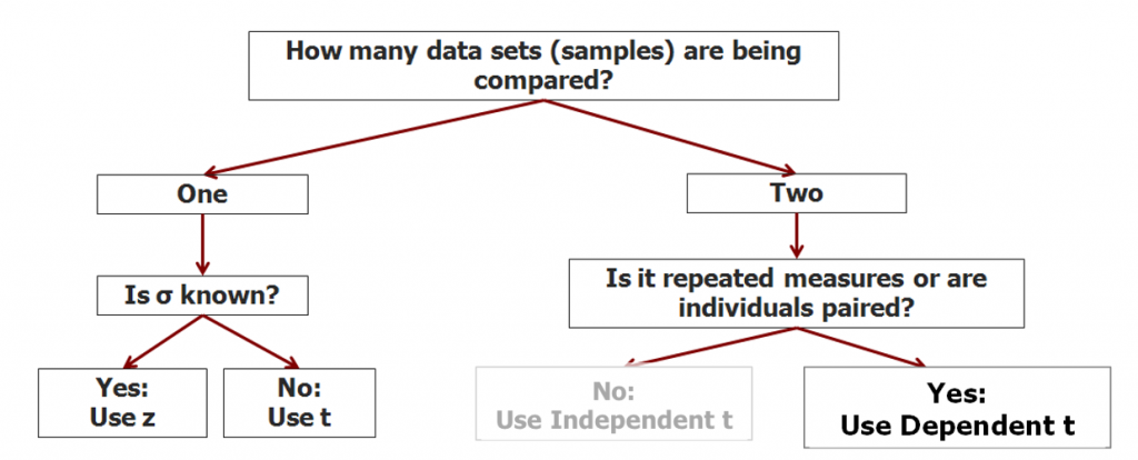
If you have two samples, and they are in some way related, like in repeated measures or matched pairs designs, that’s when we should use the dependent means t-test. In the next chapter we will add the independent means t-test to our toolbox.
Chapter Summary
In this chapter we introduced the use of the dependent means t-test in hypothesis tests for research designs such as repeated measures and matched pairs.
Key terms:
| dependent means t-test | repeated measures | matched pairs |
a test for statistical significance when comparing mean difference scores to zero in repeated measures or matched pairs designs
also known as within-subjects designs or pre-test post-test design, in which the experiment involves obtaining two separate scores for each individual in a single sample. The same participants are used in all treatment conditions.
a research design for which a dependent means t-test may be used to test for a hypothesis test; in this design two separate samples are used, but each individual in a sample is matched one-to-one with an individual in the other sample, most often matching participants on a a possible confounding variable as a way to control for the effects of that variable
