Constructing Cross-Sections
A geological cross-section is constructed by taking information from a limited number of observations that are all located along a line, and using stratigraphic principles to infer what occurs between those locations. It is rare for a geoscientist to be able to actually see all the rocks along a cross-section. At Earth’s surface rock profiles may only be exposed in sparse outcrops such as along roads or rail lines. Observations would be made at each outcrop and a stratigraphic log created from each set of observations. You saw examples of stratigraphic logs in Lab 3.
Obtaining stratigraphic information about the rocks below ground requires extra effort. Drilling rigs are used to recover rock samples from under the ground. A drill log is the record of the rock descriptions that the geoscientist has recorded for each depth interval, from which a stratigraphic log can be constructed. All the stratigraphic data are converted from height or depth relative to the ground surface to elevations above sea level. Multiple stratigraphic logs are assembled along a line and are plotted side by side. The information from one borehole or outcrop is then matched to the others by drawing lines that indicate correlations between logs.
Three broad strategies can be used for correlating between logs:
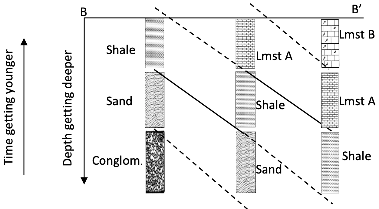
1. Lithostratigraphic correlation: Rocks of equivalent type or facies are matched (Figure 4.4).
2. Time-stratigraphic correlation: Rocks of equivalent relative (or absolute) age are matched (Figure 4.5).
3. Biostratigraphic correlation: Rocks containing the same fossil or fossil assemblage are matched, without considering rock type (Figure 4.6).
1. Lithostratigraphic Correlation
Correlation lines are drawn between neighbouring rock units to denote lithologic equivalency. They are drawn as solid lines when we are confident in the matching of one location to another. Dashed lines are used when we are inferring the correlation or the location of a contact.
In Figure 4.4 the correlation line connecting the contact between the shale and limestone A in the right-hand log and the middle log is solid because we have direct evidence of this contact in both. This correlation line dashed between the middle column and left column because we don’t have any information on where the contact is in the left-hand log. We can be confident that the contact is somewhere above the top of the recorded log in the left column, but we do not know where.
The following conditions and techniques may help with correlating rocks from one location to another based on lithology.
Similar Lithological Characteristics
If a single bed is distinctive in colour, mineral composition, grain size or structure and is laterally continuous over a wide area, it can be traced from one stratigraphic observation location to another by identifying that bed in each borehole log.
Similar Sedimentary Sequences
Multiple beds that represent a single sedimentary facies (depositional environment) can be matched from one location to another by the facies they represent. The exact bed sequence, thickness or character of individual beds within the sediment package may be slightly different at each location but together the observed sequences represent the same facies. A facies that stands out as being different from all the others can be a very reliable correlation indicator.
Fossils
As good indicators of relative age, certain fossils or fossil assemblages may be used to distinguish between beds with otherwise similar lithologies. In Figure 4.4, the limestone units may be lithologically very similar micrites, but we can distinguish between them in the field by their fossil content.
Unconformities
These are useful for correlation when the beds above and below the unconformity are found at multiple sites. Unconformities are even more useful for correlation when a rock sequence is bounded by two unconformities (above and below).
Marker Beds
Marker beds are single beds or laminae that are particularly distinct, and deposited from a distinct event. An example marker bed is an ash layer from a volcanic eruption.
Reasons for Discontinuous Strata
Sometimes rock strata will be present in one stratigraphic log and not in another. This may occur for several reasons:
a. Pinch out. The rock unit thins laterally between two locations and is not present in the adjacent stratigraphic log.
b. Lateral facies change. There was a lateral change in the depositional environment, such as from a sandy beach to a muddy tidal flat.
c. Erosion. The rock unit is absent because it has been eroded away along an unconformity (see Lab 3).
d. Deformation. A rock unit has been moved by structural deformation such as faulting.
e. Transformation. The rock has been altered by metamorphic processes such that it is no longer considered the same rock type.
2. Time-Stratigraphic Correlation
Joining rocks of the same type (lithostratigraphic correlation) does not always join together rocks of the same age. But in time-stratigraphic correlation (Figure 4.5), linking rocks of the same age is the goal.
In Figure 4.5, the conglomerate, sand, and shale at the base of each stratigraphic log are correlated because there is evidence that all were deposited at Time 1. This evidence could come from the relative position of the units at the base of the stratigraphic logs, the fossil content of the rocks, or perhaps absolute dating using radioactive isotopes. These different lithologies all belong to the same time-stratigraphic unit and time-stratigraphic correlation lines have been drawn.
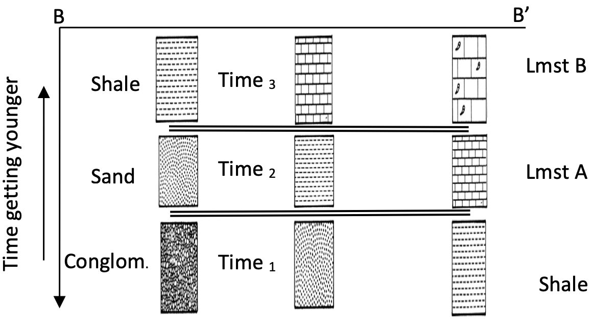
Marker beds are particularly useful for determining the boundaries of time-stratigraphic units. For example, a layer of volcanic ash will fall everywhere across the landscape at one distinct time and it would be physically distinct and easily traced from location to location.
Combining Lithostratigraphic and Time-Stratigraphic Correlation to Understand Facies Changes
During Time 2 the sand, shale and limestone A were deposited. Combining the information from Figures 4.4 and 4.5 in Figure 4.6 shows us that the sand we traced laterally in Figure 4.4 is from the same facies, but that sand was deposited at different times in different locations. The sand is said to be time-transgressive. The beach facies creating the sand was located in the middle of the section during Time 1 and had migrated to the left by Time 2. The shoreline continued to move to the left and the beach facies is no longer found in the section by Time 3.
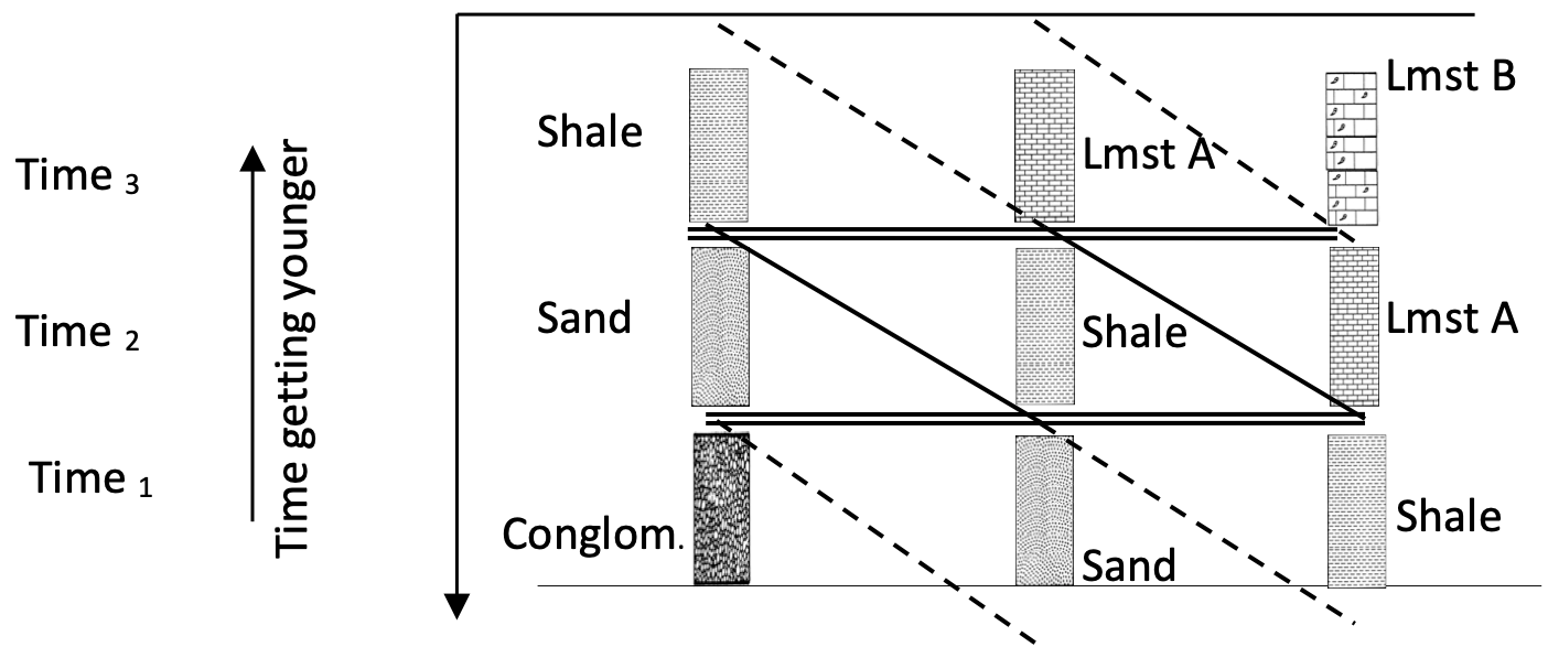
In this example, each stratigraphic log transitions from a near-shore facies to a deeper water facies over time. Using what we learned in Lab 3, we would only need one stratigraphic log to be able to say that sea level was rising. The cross-section allows us to infer that sea level was rising and that that the shoreline was located in the middle of the section at Time 1, and gradually moved left and out of the cross-section by Time 3.
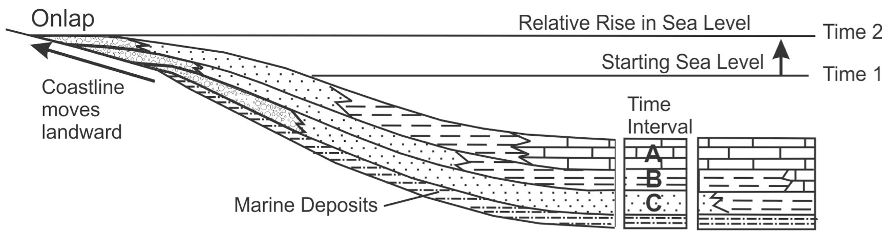
The discussion so far has been limited to the local scale, but it can be useful to consider these correlations in a larger context, at the continental scale. Figure 4.7 expands the local-scale lithostratigraphic and time-stratigraphic correlations to see the larger continental scale environmental changes between Time 1 and Time 3.
3. Biostratigraphic Correlation
The presence of a particular fossil, or assemblage of fossils, may be used to match rock units. A species that existed throughout Time 1 to Time 3, but only lived in a beach environment might be found in all the sands in our example sections. This biostratigraphic correlation is thus time-transgressive.
Next, consider a widespread fossil such as tree pollen, or ocean plankton. A short-lived species that only lived during Time 2 would allow us to trace all those rocks in our sequence and determine which of them was from Time 2. This fossil creates a marker bed because it is time specific.
Sometimes there is no one fossil with a specific age range, but a unique combination species in a fossil assemblage can be used to match beds between stratigraphic logs. You will learn more about biostratigraphy in Labs 6 to 8 as we introduce the major marine phyla in the fossil record.