Part II. Interpreting Stratigraphy in a Stratigraphic Log
Introduction
The concept of a sedimentary facies was introduced in Lab 2, and you gained experience determining facies and sedimentary environments from written descriptions of sediments, and from stratigraphic logs. You mapped facies in plan view (from above) which gives a snapshot of the spatial layout of sedimentary environments that were active at a specific time. We are now going to stay at one location in space, and observe the sediments that have been deposited at that location over time using a stratigraphic log. The changes in time observed at one location can be used to generate a spatial picture of the environment using Walther’s Law.
How to Read a Stratigraphic Log
Geoscientists draw stratigraphic logs in order to quickly relay information on rock characteristics and sequences at a single location. Standard practices may vary depending on the application (such as research on glacial landforms vs. petroleum exploration), but there are four general protocols that are followed:
1. Thickness Drawn to Scale
First, the thicknesses of each of the rock layers found along a vertical line through an outcrop, or recovered from a vertical drill core, are drawn to scale. The vertical scale on the left can be shown two ways. It can be as elevation (usually given as metres above sea level) so that each rock contact is shown at its true elevation. The scale may also be shown as depth below ground surface. Either way, the transition from one rock type to another is marked, leading to a log with the highest elevation or shallowest in the drill hole (youngest) sediments at the top and the lowest elevation or deepest in the drill hole (oldest) sediments at the bottom.
2. Grain Size Is Indicated
The grain size of the sediment at each elevation is indicated using a scale from clay to cobbles, where grain size increases along the horizontal axis (Figure 3.4). Deposits with the finest grain sizes (clay and silt) are drawn as very narrow beds, while deposits with the largest grains sizes (cobbles) are drawn much wider.
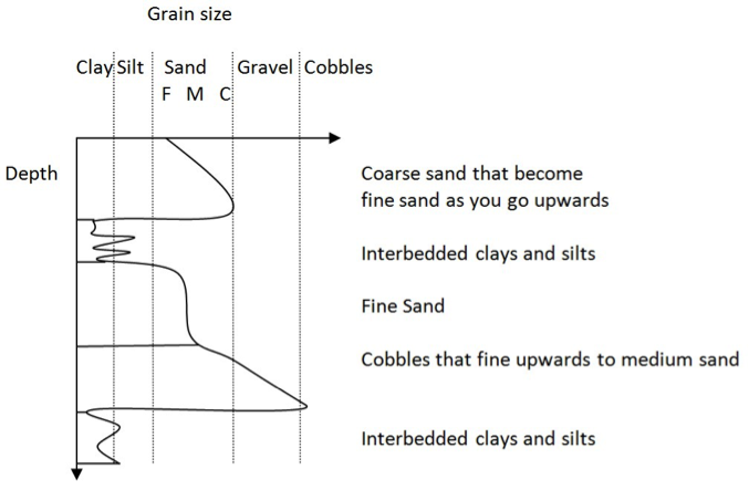
If a particular layer changes grain size from bottom to top, this can be shown by changing the location of the line between the upper and lower contacts. For example, the top layer in Figure 3.4 changes from coarse sand at its base to fine sand at the top, and therefore demonstrates a fining upward sequence (FUS). The second layer in Figure 3.4 is made up of multiple thin beds that vary between clay and silt.
3. Standard Patterns
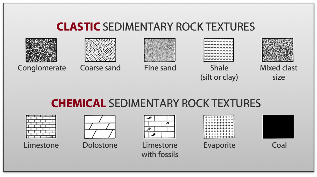
Sediment layers are filled in with standard patterns or textures based upon the rock type. This makes is easier to visually identify the rock type, particularly for chemical sedimentary rocks. Figure 3.5 shows some examples of common patterns.
4. Other Features Are Added as Patterns
Features such as the presence of fossils or the types of sedimentary structures can be added to the fill patterns.
Example
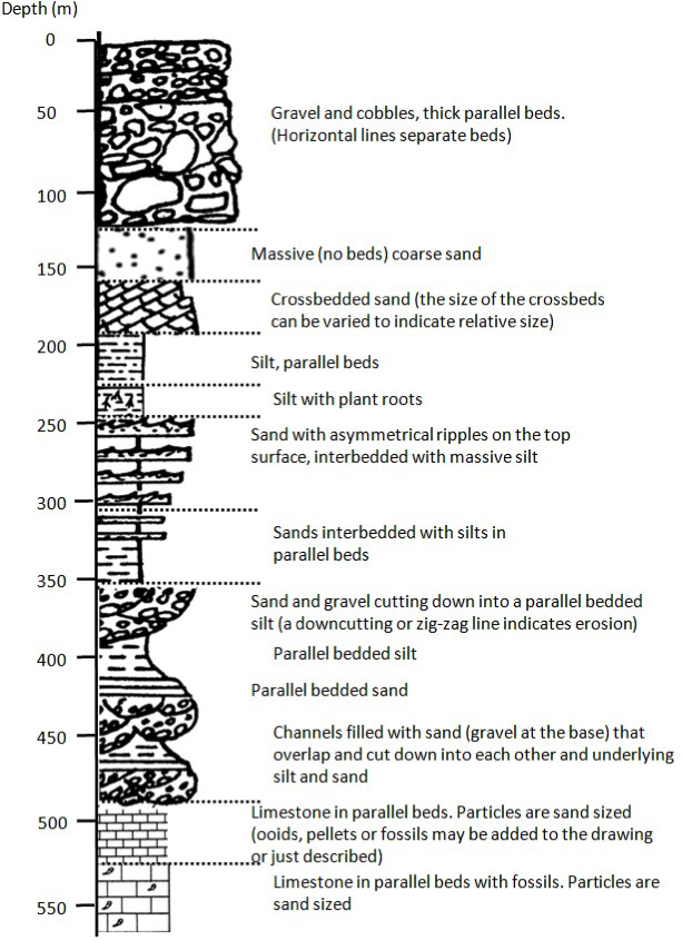
Grain size, sediment type and sedimentary structures are used together to create a complete, descriptive stratigraphic log that may be composed of numerous beds. Figure 3.6 demonstrates some examples and how to interpret them.
Stratigraphic Succession
Walther’s Law states that: “the vertical sequence of rocks mirrors the distribution of rocks commonly observed laterally.” Think back to one of the plan view photographs of depositional environments in Lab 2. At any given time, sediments are being deposited in all of these environments, so in general the sediments are getting thicker in each location.
However, also remember that the boundaries between different environments may move over time. For example, a delta may gradually prograde (advance sideways) out further into the sea. or a barrier island may gradually lengthen down the coast. Over time, the exact spatial locations of the boundaries of different environments will change, but their relative positions may not. The delta environment is still downstream of the meandering river, and it is still higher up the transport sequence than the shelf environment.
There are two ways that the sediments at a point can shift character:
1. Lateral Migration
The boundaries between sedimentary environments, and hence the sedimentary facies they create, are naturally migrating laterally within an otherwise similar environment or climate as sediments fill the depositional basin.
Think about it this way: imagine placing your hand on the table, and then a plan view map of depositional environments on top of your hand. Next, slide the map to one side without moving your hand. The depositional environment above a particular point on your hand changes as you slide the paper. This mimics what might happen as a delta deposits more and more sediment and moves laterally further into the ocean. The spot above your hand was originally depositing sediments of a certain facies (such as a shelf), but as the delta’s boundaries shifted laterally, different sediments began depositing at that location. This appears in the rock record as marine shelf deposits with a delta facies on top of them. Above that, the meandering river facies might appear as the shoreline moved past your point on the table.
2. Sea Level Change
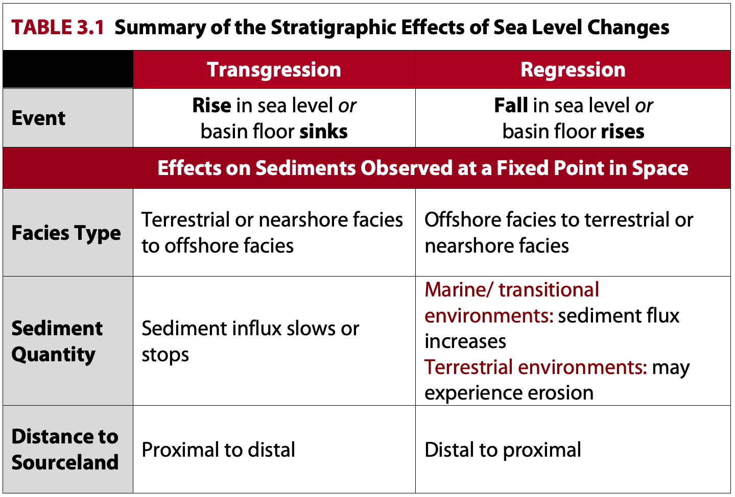
The other mechanism that changes the locations of depositional environments is if there is a change in sea level. This causes a lateral shift in all the facies boundaries. Rising sea levels (transgression) mean that each location on the map that was already in the ocean is now deeper under water, or a location may now be submerged when it was not before. The gradients of rivers will re-adjust to the new sea level, as will the terrestrial facies. Falling sea levels (regression) mean formerly submerged sediments may now be terrestrial and subject to erosion, and other ocean sediments are under shallower water. The overall effects are summarized in Table 3.1, and each is described in more detail below.
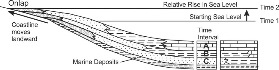
Transgression
Rising sea levels deposit marine sediment on older rock previously exposed on land (Figure 3.7). Transgression is accompanied by a fining upwards sequence of grain size. In Figure 3.7, the stratigraphic column was located close to the shoreline at Time 1, depositing coarser clastic sediment such as sands (C). Sea level began to rise relative to this point, increasing the water depth, and thus resulting in the deposition of silts (B). Micrites (A), which form far from sediment sourcelands in the deep shelf or ocean, deposit on top of (B) by Time 2.
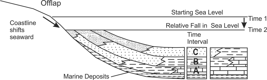
Regression
Falling sea level may cause erosion of sediments that were once covered by water, and results in a seaward shift in the boundary between marine and non-marine deposits (Figure 3.8). Regression results in a coarsening upwards sequence of grain size at an observation point offshore. In the figure below, the stratigraphic column was located far from land at Time 1, and the sediments accumulating were deep ocean micrites (A). As sea level falls, the stratigraphic column is progressively closer to shore and water depth decreases. The sediment changes to fine siltstones (B) as the sediment source area becomes closer, then to coarser clastic sediment such as sands (C). On land, the marine sediments no longer accumulate. In some circumstances, terrestrial sediments such as alluvial sediments may still accumulate on top. Or, the marine sediments will be exposed to weathering forces and may begin to erode. If sea level were to rise once more, this would be the site of a regional unconformity.
Causes of Sea Level Change
The causes of the rise and fall of sea level are complex and interrelated.
Short-Term Sea Level Change (Thousands of Years)
1. Melting and Freezing of Ice on Land
Global changes can be generated by the forming or melting of glaciers and ice caps. Ice sheets are created when ice forms on land during glacial periods and covers a large area of a continent (e.g., Greenland, Antarctica), thus removing water from the ocean and lowering sea levels (regression). Melting of this land-based ice causes sea level to rise (transgression).
The amount of water tied up globally in glaciers and ice caps has varied over Earth’s history and there are been five major global glacial periods. The incorporation or release of water held in ice caps can create eustatic (global) sea level change.
2. Thermal Expansion of Ocean Water
When a liquid is heated, its volume increases (this is called thermal expansion), and volume decreases when the liquid cools. This is the principle behind liquid-based thermometers such as those filled with red alcohol. We know how much the liquid will expand with a given change in temperature, and thus how much of the tube the liquid will fill. Marking off those levels gives us the temperature scale.
Seawater also responds to temperature change, and thus short-term changes can also be brought about by thermal expansion/contraction of the ocean as its mean temperature rises and falls. This enhances the effects of a glacial period, where the same cold climate conditions that form glaciers also cause the water in the ocean to shrink. Thermal expansion of the warming global ocean over the next century will contribute to a significant proportion of the expected rise in global sea levels brought about by climate change. The melting land-based ice in Antarctica and Greenland will contribute the rest.
Long-Term Sea Level Change (Millions of Years)
1. Local Changes due to Regional Tectonics
Over millions of years, changes in local sea level relative to the land can be created by local tectonic events such as mountain building, faulting, or igneous intrusions that deform or change the land surface in a region. This may cause the basin floor to rise or sink relative to an unchanging global sea level. These effects would be observed just within the area affected by the tectonic changes.
2. Global Changes due to Mid-Ocean Ridges
Changes in global sea level are associated with the global rate of mid-ocean ridge spreading. Earth’s oceanic lithospheric plates are always being created and destroyed, and their arrangements and ages change over time. A global plate configuration with many small, young oceanic plates and many active spreading centres results in the average volume of the deep ocean being lower because deep ocean space is being occupied by the many ridges. Younger plates have also had less time to cool and become denser, and tend to float higher on the underlying mantle. The average ocean floor is therefore shallower relative to the continents. Again, this means there is less deep ocean volume, and sea water will rise onto the continents. (Think about adding rocks to a bucket of water, and watching the water level become higher in the bucket because the rocks are displacing the water.)
The opposite is true when there are fewer, larger, older ocean lithosphere plates and an overall shorter length of spreading ridges globally. The volume of the ocean occupied by spreading ridges is smaller, and the older plates are colder and denser and sink lower relative to the continents where they are furthest from the ocean ridges. The volume of the global deep oceans increases and global sea levels fall relative to the continents. (In other words, there is more room for water in the ocean, so it doesn’t have to spill onto land.)
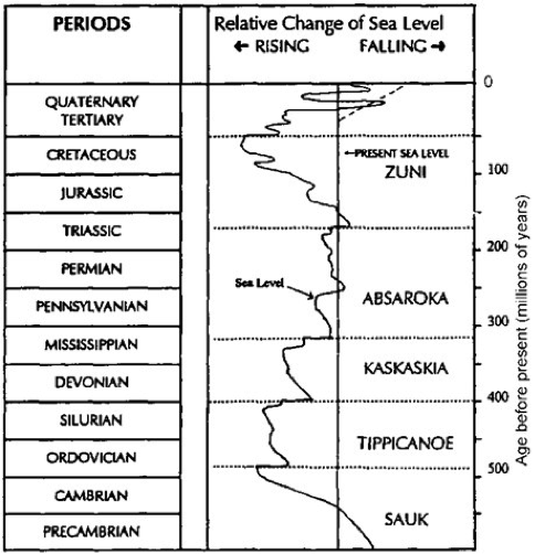
Eustatic Curves Illustrate Sea-Level Change
The changes in global (or local) sea level over time can be plotted using a eustatic curve. Figure 3.9 shows the global average changes in sea level over the last 600 million years. Imagine a beach location. When the curve moves to the left (transgression, rising sea level), that beach would be under deeper water, and the sediments would move toward deeper ocean facies.
In contrast, when the curve moves to the right indicating falling sea levels (regression), the beach sediments would be higher on land, and either eroding or being covered by terrestrial sediments such as alluvial fan sequences.
A body of sediment with distinctive physical, chemical and biological attributes deposited in a specific depositional environment.
The vertical sequence of rocks mirrors the distribution of rocks commonly observed laterally. In other words, the horizontal gradations in depositional environments that you learned about in Lab 2 are repeated vertically as environmental conditions at a location change over time (e.g. sea level rise). This applies when the rock record is continuous and has no gaps in time.