15 Equilibrium Reactions

When the concentrations of reactants and products become constant, the system is said to have reached a point of equilibrium. The equilibrium state is dynamic. At equilibrium, the reactions are not stopped, but rather the rates of opposing reactions have become equal such that concentrations of chemical species do not change.

Laboratory kinetic studies may be performed on reactions far from equilibrium where products are in low concentration and the reverse reactions are not important (this is what we considered previously).

$C{O}_{(g)}+H_2{O}_{(g)}\to C{O}_{2(g)}+H_{2(g)}$

Closer to equilibrium however we must take these reverse reactions into account.

$C{O}_{(g)}+H_2{O}_{(g)}\rightleftharpoons C{O}_{2(g)}+H_{2(g)}$

Equilibrium Constant

Consider a system with the following reaction:

$A\rightleftharpoons B$

Let’s say the system is composed of 2 first-order reactions:

Forward reaction: $A\to B$, where the reaction rate is expressed by: $r=k_r\times [A]$
Reverse reaction: $B\to A$, where the reaction rate is expressed by: $r^{\prime }=k_r^{\prime }\times [B]$

Net rate of change in $[A]$ considering both reactions is:

$\frac{d[A]}{dt}=r^{\prime }-r=k_r^{\prime }\times [B]-k_r\times [A]$

If the initial concentration of A is $[A{]}_0$ and no B is present, then at all times: $[A]+[B]=[A{]}_0$. Using this in the equation above:

$$\begin{array}{rl}\frac{d[A]}{dt}& =k_r^{\prime }[B]-k_r[A]\\ & =k_r^{\prime }([A{]}_0-[A])-k_r[A]\\ & =k_r^{\prime }[A{]}_0-(k_r+k_r^{\prime })[A]\end{array}$$

This is what is known as an ordinary differential equation, as $[A]$ is both a differential and a separate term. You may not know how to solve these equations and do not need to know this for this course. However, if we were to solve this ordinary differential equation, we would get the following:

$[A]=\frac{k_r^{\prime }+k_r{e}^{-(k_r^{\prime }+kr)t}}{k_r^{\prime }+k_r}[A{]}_0$

Using the expression for $[A]$ above, $[B]=[A{]}_0-[A]$, taking arbitrary values of $k_r=0.693$ and $k_r^{\prime }=0.262$, the following graph is produced:

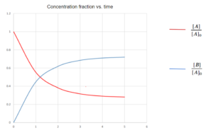As you can see from the graph, the concentrations change less over time. After a long time, they should reach a state of equilibrium. The length of time to reach equilibrium (or close to it) will depend on the reaction rates.

As $t\to \mathrm{\infty }$, we approach equilibrium and we get the following:

$[A{]}_{eq}=\frac{k_r^{\prime }+k_r{e}^{-(k_r^{\prime }+kr)t}}{k_r^{\prime }+k_r}[A{]}_0=\frac{k_r^{\prime }}{k_r^{\prime }+k_r}[A{]}_0$

and
$[B{]}_{eq}=[A{]}_0-[A{]}_{eq}=\frac{k_r}{k_r^{\prime }+k_r}[A{]}_0$

The equilibrium constant in this example is defined as:

At equilibrium, the rates of forward and reverse reactions should be the same (meaning no change in overall concentrations), so it makes sense that when we rearrange this we get:

Consider another system with the following reaction:

$A+B\rightleftharpoons C$

Forward reaction: $A+B\to C$, where the forward reaction rate is expressed by: $r=k_r[A][B]$

Reverse reaction: $C\to A+B$, where the reverse reaction rate is expressed by: $r^{\prime }=k_r^{\prime }[C]$

Here, in equilibrium we have:

$r=r^{\prime }=k_r[A{]}_{eq}[B{]}_{eq}=k_r^{\prime }[C{]}_{eq}$

The equilibrium constant is defined as dimensionless, so here is where the $c^{\theta }$ terms make a difference. The equilibrium constant can be espressed as:

$K=\frac{[C{]}_{eq}/c^{\theta }}{[A{]}_{eq}/c^{\theta }\times [B{]}_{eq}/c^{\theta }}=(\frac{[C]}{[A][B]}{)}_{eq}=\frac{k_r}{k_r^{\prime }}{c}^{\theta }$

Recall that $k_r$ and $k_r^{\prime }$ here will have different units, so the $c^{\theta }$ term ensures that these become dimensionless when one is divided by the other.

References

[1] Chemistry LibreTexts. 2020. Characteristics of the Equilibrium State. [online] Available at: <https://chem.libretexts.org/Bookshelves/Physical_and_Theoretical_Chemistry_Textbook_Maps/Supplemental_Modules_(Physical_and_Theoretical_Chemistry)/Equilibria/Chemical_Equilibria/Principles_of_Chemical_Equilibria/Principles_of_Chemical_Equilibrium/Characteristics_Of_The_Equilibrium_State> [Accessed 24 April, 2020].
Feedback/Errata