6. Entropy and the Second Law of Thermodynamics
6.9 The second law of thermodynamics for open systems
Entropy can be transferred to a system via two mechanisms: (1) heat transfer and (2) mass transfer. For open systems, the second law of thermodynamics is often written in the rate form; therefore, we are interested in the time rate of entropy transfer due to heat transfer and mass transfer.
[latex]\dot{S}_{heat} =\dfrac{dS_{heat}}{dt} \cong \displaystyle\sum\dfrac{\dot{Q}_k}{T_k}[/latex]
[latex]\dot{S}_{mass} = \displaystyle\sum\dfrac{dS_{mass}}{dt} = \displaystyle \sum \dot{m}_{k}s_{k}[/latex]
where
[latex]\dot{m}[/latex]: rate of mass transfer
[latex]\dot{Q}_k[/latex]: rate of heat transfer via the location [latex]k[/latex] of the system boundary, which is at a temperature of [latex]T_k[/latex] in Kelvin
[latex]\dot{S}_{heat}[/latex]: time rate of entropy transfer due to heat transfer
[latex]\dot{S}_{mass}[/latex]: time rate of entropy transfer that accompanies the mass transfer into or out of a control volume
[latex]s_k[/latex]: specific entropy of the fluid
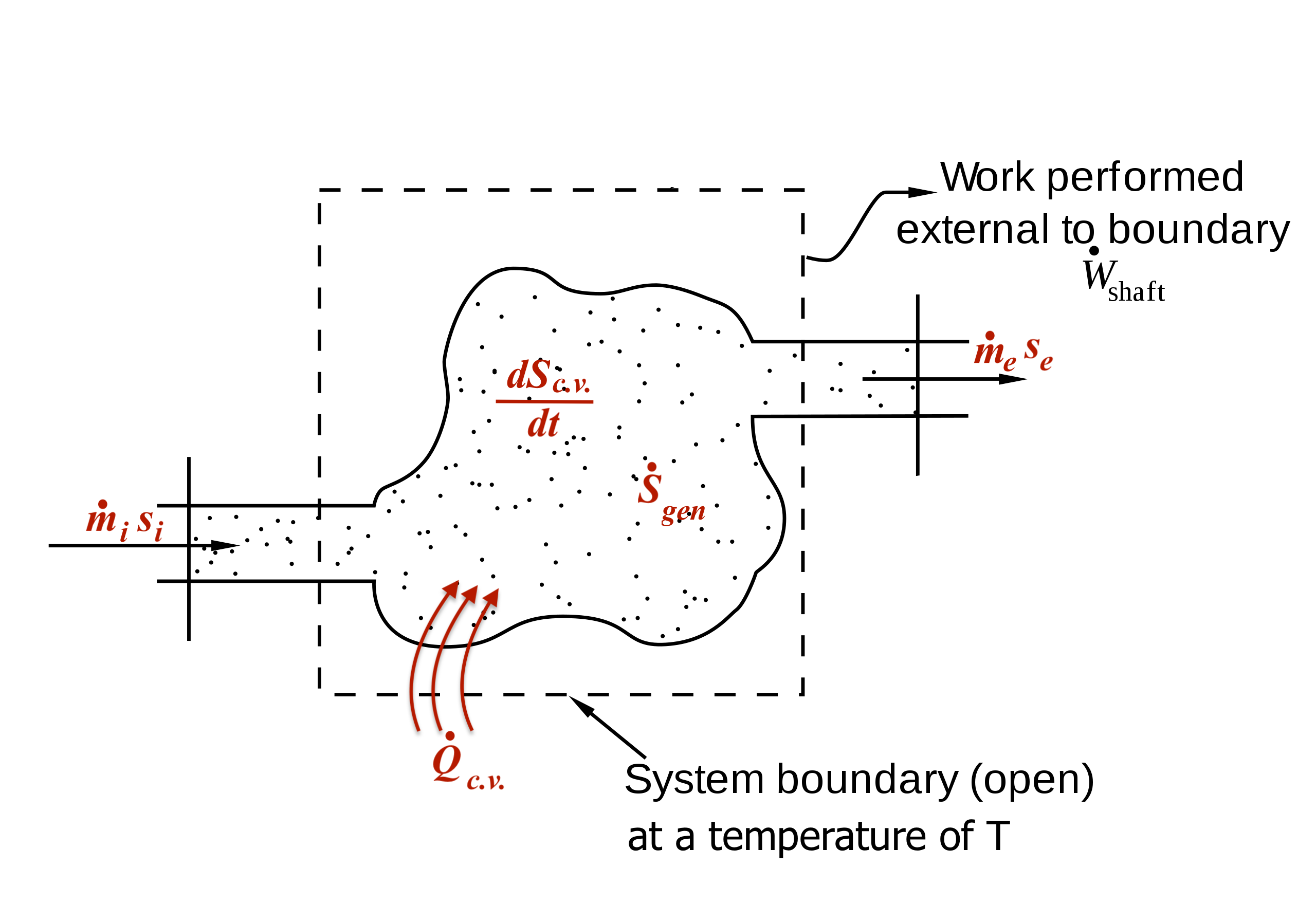
Applying the entropy balance equation, [latex]\Delta \rm {entropy= + in - out + gen}[/latex], to a control volume, see Figure 6.9.1, we can write the following equations:
- General equation for both steady and transient flow devices
[latex]\dfrac{{{dS}}_{{c}.{v}.}}{{dt}}=\displaystyle\left(\sum{{\dot{{m}}}_{i}{s}_{i}}+\displaystyle\sum\frac{{\dot{{Q}}}_{{c}.{v}.}}{{T}}\right)-\displaystyle\left(\sum{{\dot{{m}}}_{e}{s}_{e}}\right)+\displaystyle{\dot{{S}}}_{{gen}}\ \ \ \ \ \ ({\dot{{S}}}_{{gen}} \ge 0)[/latex]
- For steady-state, steady-flow devices, [latex]\dfrac{{dS}_{c.v.}}{dt}=0[/latex]; therefore,
[latex]\displaystyle \sum{{\dot{{m}}}_{e}{s}_{e}}-\sum{{\dot{{m}}}_{i}{s}_{i}}=\displaystyle \sum\dfrac{{\dot{{Q}}}_{{c}.{v}.}}{{T}}+{\dot{{S}}}_{{gen}}\ \ \ \ \ \ ({\dot{{S}}}_{{gen}} \ge 0)[/latex]
- For steady and isentropic flow devices, [latex]\dot{Q}_{c.v.}=0[/latex] and [latex]\dot S_{gen}=0[/latex]; therefore,
[latex]\displaystyle\sum{{\dot{{m}}}_{e}{s}_{e}}=\displaystyle\sum{{\dot{{m}}}_{i}{s}_{i}}[/latex]
where
[latex]\dot{m}[/latex]: rate of mass transfer of the fluid entering or leaving the control volume via the inlet [latex]i[/latex] or exit [latex]e[/latex], in kg/s
[latex]\dot{Q}_{c.v.}[/latex]: rate of heat transfer into the control volume via the system boundary (at a constant [latex]T[/latex]), in kW
[latex]S_{c.v.}[/latex]: entropy in the control volume, in kJ/K
[latex]\dfrac{{dS}_{c.v.}}{dt}[/latex]: time rate of change of entropy in the control volume, in kW/K
[latex]\dot S_{gen}[/latex]: time rate of entropy generation in the process, in kW/K
[latex]s[/latex]: specific entropy of the fluid entering or leaving the control volume via the inlet [latex]i[/latex] or exit [latex]e[/latex], in kJ/kgK
[latex]T[/latex]: absolute temperature of the system boundary, in Kelvin
Example 1
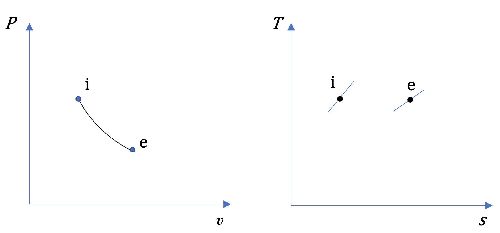
The diagrams in Figure 6.9.e1 show a reversible process in a steady-state, single flow of air. The letters i and e represent the initial and final states, respectively. Treat air as an ideal gas and assume ΔKE=ΔPE=0. Are the change in specific enthalpy Δh=he−hi, specific work w, and specific heat transfer q positive, zero, or negative values? What is the relation between w and q?
Solution:
The specific work can be evaluated mathematically and graphically.
(1) Mathematically,
[latex]\because v_{e} > v_{i}[/latex]
[latex]\therefore w = \displaystyle\int_{i}^{e}{Pd{v}\ } >\ 0[/latex]
(2) Graphically, the specific work is the area under the process curve in the [latex]P-v[/latex] diagram; therefore [latex]w[/latex] is positive, see Figure 6.9.e2.
In a similar fashion, the specific heat transfer can also be evaluated graphically and mathematically.
(1) Graphically,
[latex]\because ds=\left(\displaystyle\frac{\delta q}{T}\right)_{rev}[/latex]
[latex]\therefore q_{rev} = \displaystyle \int_{i}^{e}{Tds} = T(s_e-s_i)\ >\ 0[/latex]
For a reversible process, the area under the process curve in the [latex]T-s[/latex] diagram represents the specific heat transfer of the reversible process; therefore [latex]q=q_{rev}[/latex] is positive, see Figure 6.9.e2.
(2) The same conclusion, [latex]q_{rev}>0[/latex], can also be derived from the second law of thermodynamics mathematically, as follows.
[latex]\dot{m}(s_e-s_i)=\displaystyle\sum\frac{\dot{Q}}{T_{surr}}+\dot{S}_{gen}[/latex]
For a reversible process, [latex]\dot{S}_{gen}[/latex]= 0, and the fluid is assumed to be always in thermal equilibrium with the system boundary, or [latex]T = T_{surr}[/latex]; therefore,
[latex]q_{rev} = \dfrac{\dot{Q}}{\dot{m}} = T(s_e-s_i) > 0[/latex]
The change in specific enthalpy can then be evaluated. For an ideal gas,
[latex]\Delta h = h_e - h_i = C_p(T_e - T_i)[/latex]
[latex]\because T_e = T_i[/latex]
[latex]\therefore h_e = h_i[/latex] and [latex]\Delta h =0[/latex]
Now, we can determine the relation between [latex]w[/latex] and [latex]q_{rev}[/latex] from the first law of thermodynamics for control volumes.
[latex]\because \dot{m}( h_e - h_i ) = \dot{Q}_{rev} - \dot{W} = 0[/latex]
[latex]\therefore \dot{Q}_{rev} = \dot{W}[/latex]
[latex]\therefore q_{rev} = w[/latex]
In this reversible process, the specific heat transfer and specific work must be the same. Graphically, the two areas under the [latex]P-v[/latex] and [latex]T-s[/latex] diagrams must be the same.

Practice Problems
Media Attributions
- Entropy transfers and entropy generation through a C.V. © Pbroks13 is licensed under a Public Domain license
An isentropic process refers to a process that is reversible and adiabatic. The entropy remains constant in an isentropic process.
