2. Thermodynamic Properties of a Pure Substance
2.4 Thermodynamic tables
Thermodynamic tables are commonly used to determine the properties of a substance at a given state. This book includes the tables for four pure substances: water, ammonia, R134a, and carbon dioxide. The data in these tables are obtained from NIST Chemistry WebBook, SRD 69, which consists of the thermophysical properties of various common fluids.
Appendix A: Thermodynamic Properties of Water
Appendix B: Thermodynamic Properties of Ammonia
Appendix C: Thermodynamic Properties of R134a
Appendix D: Thermodynamic Properties of Carbon Dioxide
Tables A1, B1, C1, and D1 are the tables for the saturated fluids. They are used to find the properties of the corresponding fluids in saturated liquid, saturated vapour, and two-phase regions. Tables A2, B2, C2, and D2 are the superheated vapour tables for finding the properties of the fluids in the superheated vapour region. Table A3 is the compressed liquid table for water.
In these tables, the specific volume, specific internal energy, specific enthalpy, and specific entropy are tabulated as functions of the pressure and temperature. Among those thermodynamic properties, [latex]P[/latex], [latex]T[/latex], and [latex]v[/latex] are measurable properties, and [latex]u[/latex], [latex]h[/latex], and [latex]s[/latex] cannot be measured directly. They are calculated with respect to predefined reference states. The reference states used for different tables in this book are stated in Appendices A to D.
It is important to be aware that thermodynamic tables can be generated with respect to different reference states, which means that the values of specific internal energy [latex]u[/latex], specific enthalpy [latex]h[/latex], and specific entropy [latex]s[/latex] can vary depending on the source of the tables. Additionally, in most thermodynamic analyses, we are concerned with the changes in these specific properties, such as [latex]\Delta u[/latex], [latex]\Delta h[/latex], and [latex]\Delta s[/latex]. Therefore, it is important to use tables from a single source in order to ensure that consistent values of [latex]u[/latex], [latex]h[/latex], and [latex]s[/latex] are used in the analysis. Using tables from different sources in calculations can lead to incorrect or misleading conclusions.
When using thermodynamic tables, we will need to consider the following two questions: (1) how many independent variables are required to fix the state of a fluid? and (2) how the phase of a fluid is determined? is it a compressed liquid, superheated vapour, or two-phase liquid-vapour mixture?
By examining the tables in Appendices A to D, you probably have already noticed that all properties in these tables are intensive properties. For a non-reactive system in thermodynamic equilibrium, the Gibbs phase rule indicates that the number of independent, intensive properties of the system can be found as
[latex]f=c+2-p[/latex]
where
[latex]f[/latex]: the number of independent, intensive properties of the system that are needed to fix the state of the system. It is also called the degree of freedom of the system.
[latex]c[/latex]: the number of components of the system. For a pure substance, [latex]c=1[/latex].
[latex]p[/latex]: the number of phases of the system. For a single-phase system, [latex]p=1[/latex]. If a system is in a two-phase region, [latex]p=2[/latex].
For a single-phase system of a pure substance, [latex]c=1[/latex], [latex]p=1[/latex]; therefore, [latex]f=2[/latex]. This means that two independent, intensive properties are required to fix the state of the system. In other words, if any TWO independent, intensive properties from this list, [latex]P[/latex], [latex]T[/latex], [latex]v[/latex], [latex]u[/latex], [latex]h[/latex], [latex]s[/latex], are known, then the remaining intensive properties can be determined from the thermodynamic tables.
For a pure substance in a two-phase, saturated region, such as a mixture of saturated liquid water and saturated water vapour, [latex]c=1[/latex], [latex]p=2[/latex]; therefore, [latex]f=1[/latex]. This means that the system is of one-degree of freedom; if one independent, intensive property, such as the saturated temperature, [latex]T_{sat}[/latex], or the saturated pressure, [latex]P_{sat}[/latex] of the mixture is fixed, all other intensive properties of the saturated mixture can be found from the thermodynamic tables, which include [latex]P_{sat}[/latex] (or [latex]T_{sat}[/latex]), [latex]v_f[/latex], [latex]v_g[/latex], [latex]u_f[/latex], [latex]u_g[/latex], [latex]h_f[/latex], [latex]h_g[/latex], [latex]s_f[/latex], and [latex]s_g[/latex]. With the quality [latex]x[/latex], we can calculate the specific properties, [latex]v[/latex], [latex]u[/latex], [latex]h[/latex], and [latex]s[/latex] of the saturated mixture. In summary, for a pure substance in a two-phase, saturated region, if any TWO independent, intensive properties from this list, [latex]P[/latex], [latex]T[/latex], [latex]v[/latex], [latex]u[/latex], [latex]h[/latex], [latex]s[/latex], and [latex]x[/latex], are known, then the remaining intensive properties can be calculated from the thermodynamic tables.
The following flow charts demonstrate four common scenarios and the corresponding procedures of finding thermodynamic properties.
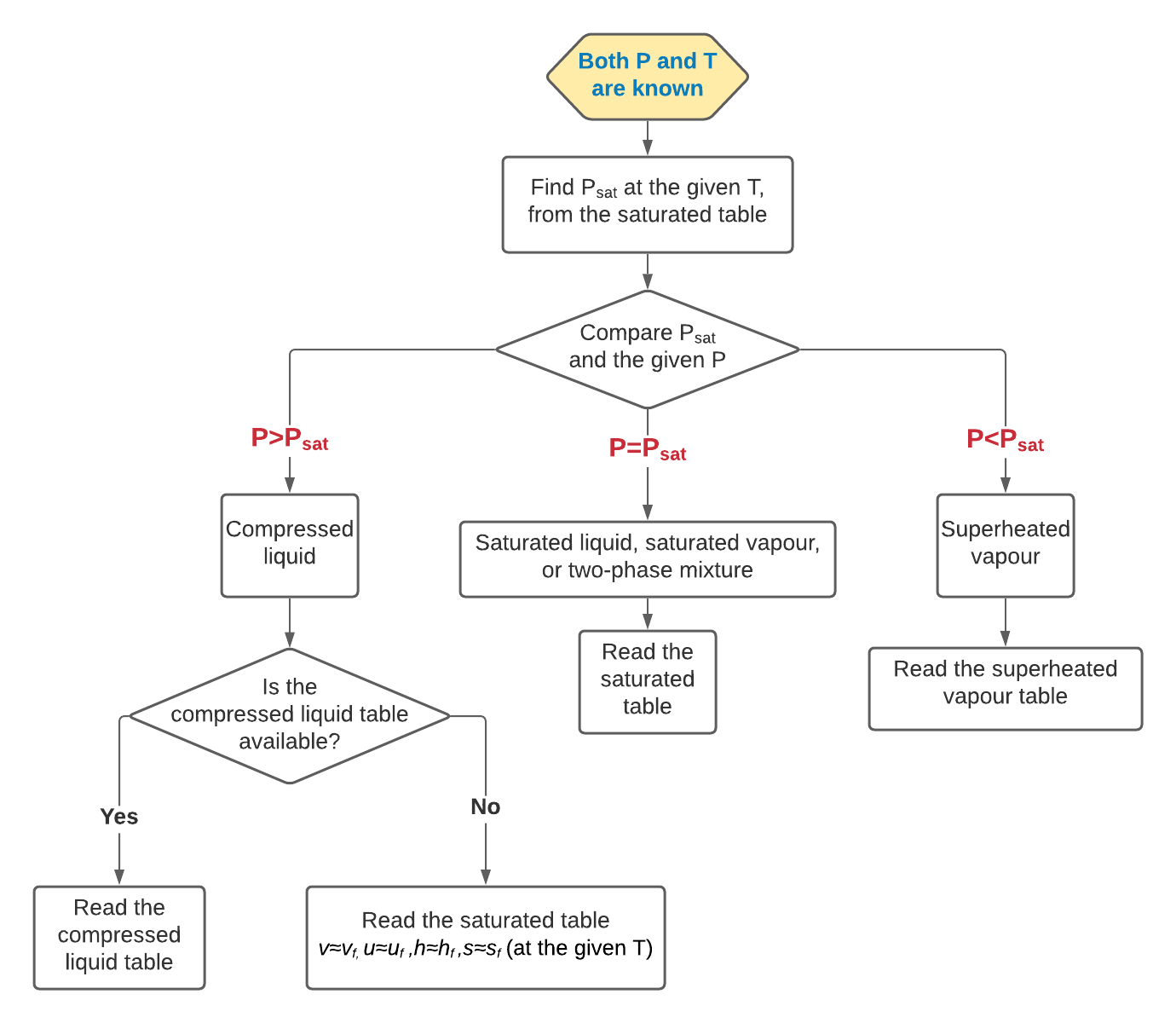
Case 1: both T and P are given. You may draw a [latex]P-T[/latex] diagram (see Figure 2.3.2) to help you better understand the flow chart in Figure 2.4.1.
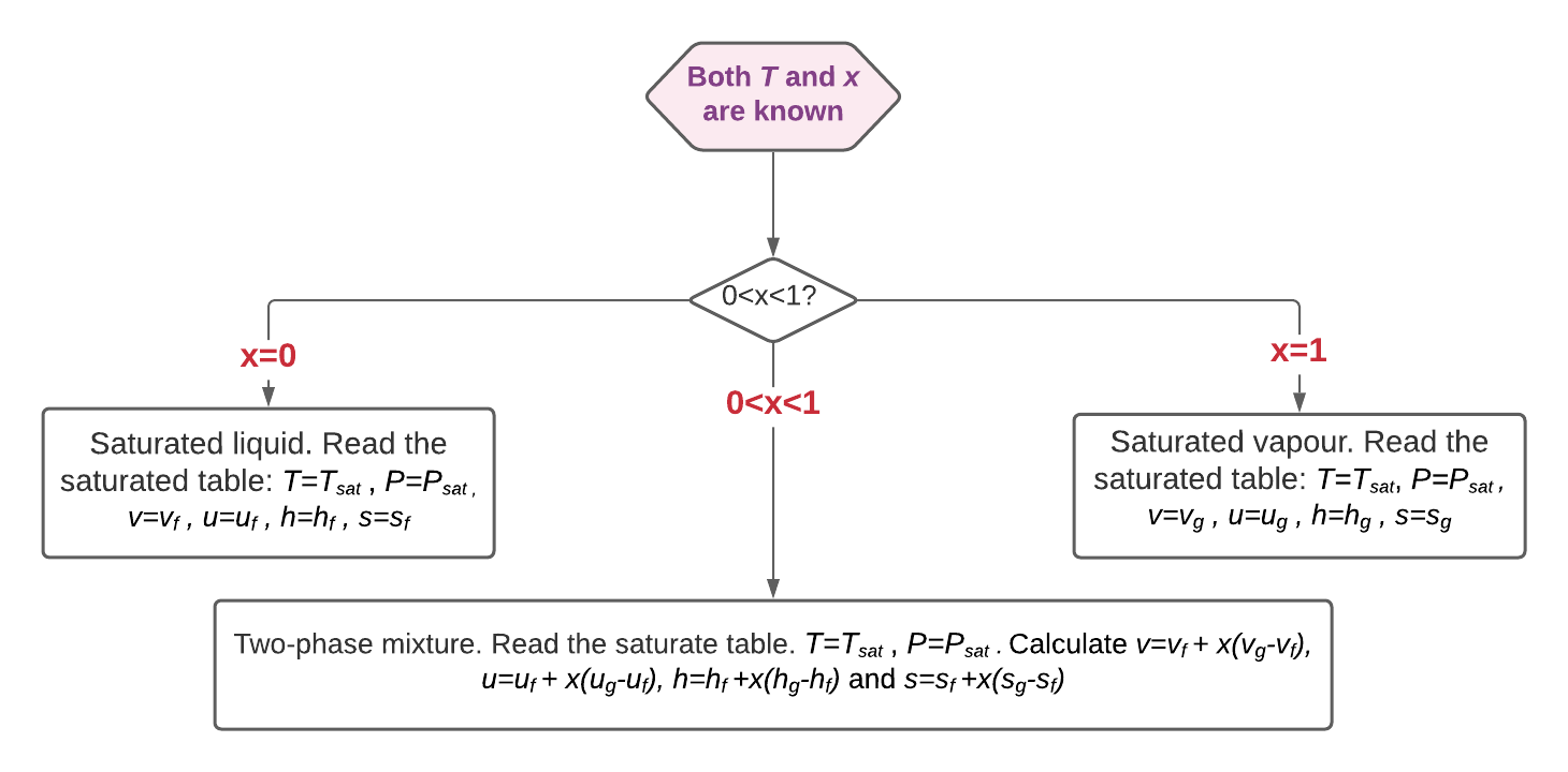
Case 2: both T and x are given. You may draw a [latex]T-v[/latex] diagram (see Figure 2.3.4) to help you better understand the flow chart in Figure 2.4.2.
Case 3: both T and v are given. You may draw a [latex]T-v[/latex] diagram (see Figure 2.3.4) to help you better understand the flow chart in Figure 2.4.3.
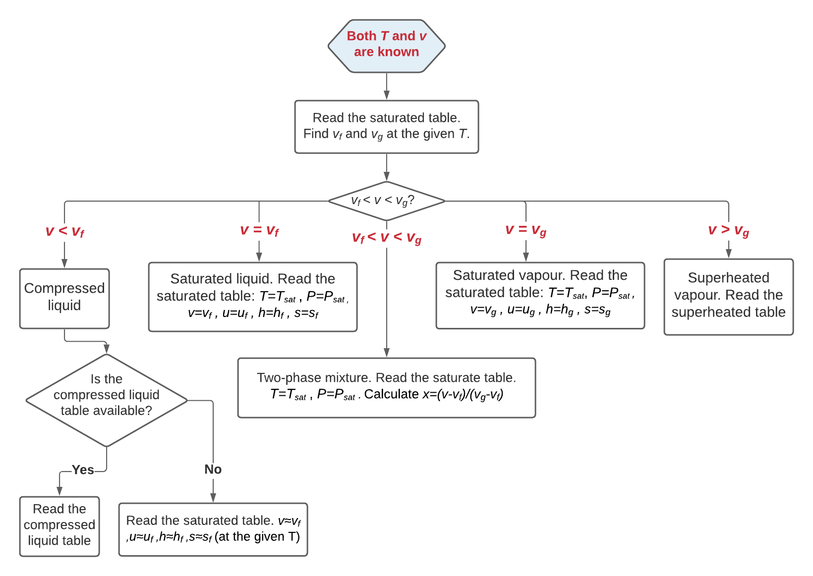
Case 4: temperature T and one of u, h and s are given. The procedure is exactly the same as for case 3. Replace [latex]v[/latex] with the given [latex]u[/latex], [latex]h[/latex], or [latex]s[/latex] in the flow chart, Figure 2.4.3.
The compressed liquid table is presented only for water in the pressure range of 0.5-50 MPa in this book. When the compressed liquid tables are not available for a specific fluid or in a specific range, the saturated liquid properties at the same temperature may be used as an approximation, i.e., [latex]v\approx\ v_{f@T}[/latex], [latex]u\approx\ u_{f@T}[/latex], [latex]h\approx\ h_{f@T}[/latex], and [latex]s\approx\ s_{f@T}[/latex].
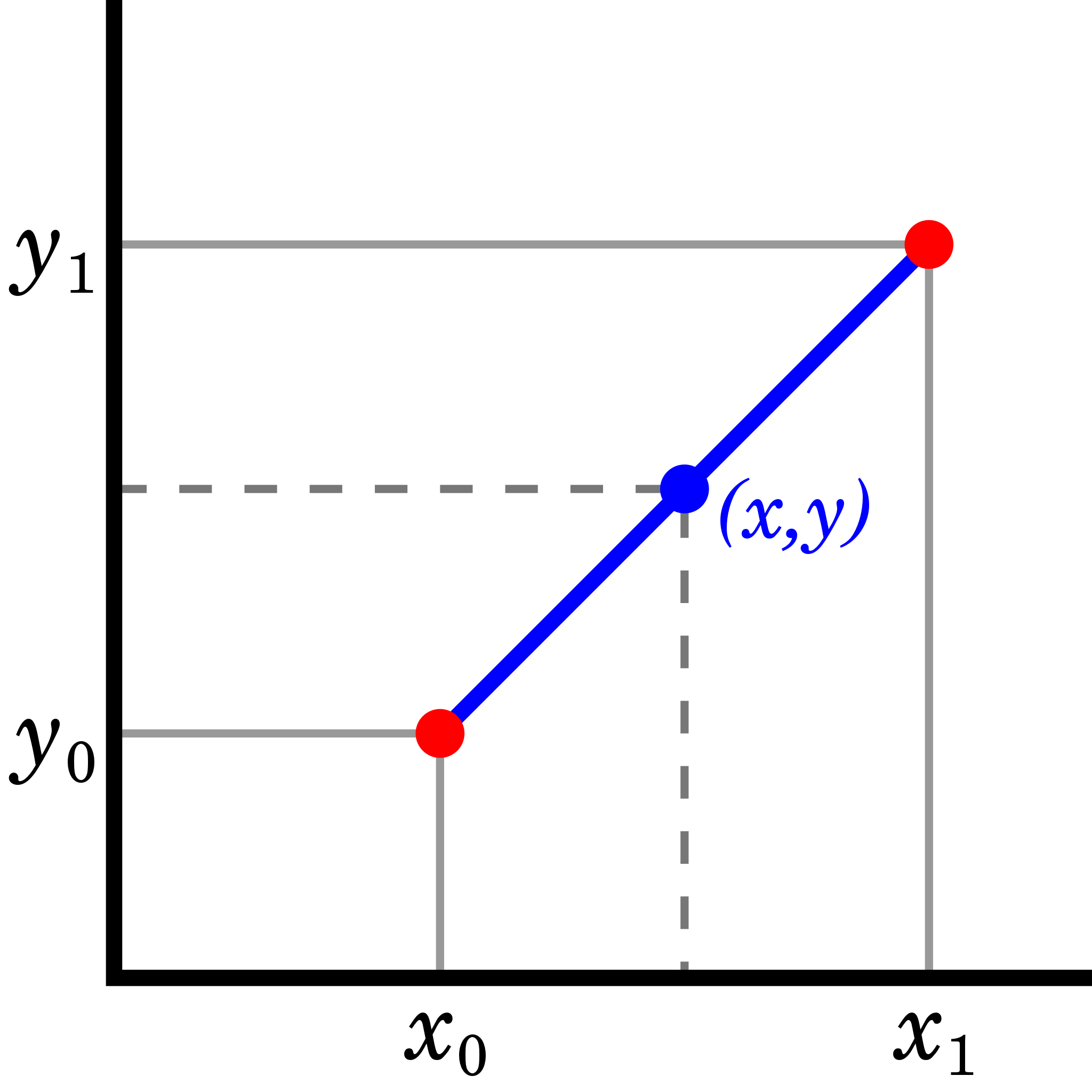
The tables in Appendices A to D are presented with a small temperature increment. Linear interpolations, see Figure 2.4.4, are often used if the given temperature or other properties cannot be found directly from these tables.
[latex]y=y_0+\left( x-x_0 \right) \dfrac{y_1-y_0}{x_1-x_0}[/latex]
where [latex]\left( x, y \right)[/latex] is the state, at which the property [latex]x[/latex] is known and the property [latex]y[/latex] is to be found. [latex]\left( x_0, y_0 \right)[/latex] and [latex]\left( x_1, y_1 \right)[/latex] indicate the properties of two known states, between which the unknown state [latex]\left( x, y \right)[/latex] is located. To improve the accuracy, the two states should be selected as close as possible to the unknown state.
The following examples demonstrate how to use these tables to find the properties of a compressed liquid, superheated vapour, and liquid-vapour mixture.
Example 1
Determine the properties of water at T=150oC and P=100 kPa.
Solution:
-
Both temperature and pressure are given for water. Use the flow chart for case 1, Figure 2.4.1.
-
From Table A1: at T=150oC, Psat = 0.47617 MPa = 476.17 kPa.
-
Because P=100 kPa < 476.17 kPa, or P < Psat , water at this state is a superheated vapour.
-
From Table A2: at T=150oC and P=100 kPa,
v = 1.93665 m3/kg, u = 2582.94 kJ/kg
h = 2776.60 kJ/kg, s = 7.6148 kJ/kgK
Example 2
Determine the properties of ammonia at T=0oC and v =0.2 m3/kg.
Solution:
-
Both T and v are given for ammonia. Use the flow chart for case 3, Figure 2.4.3.
-
From Table B1: at T=0oC, vf =0.001566 m3/kg and vg = 0.289297 m3/kg.
-
Because vf < v < vg , ammonia at this state is a liquid-vapour two-phase mixture. Its pressure and quality are
[latex]P=P_{sat}=0.42939 \ \rm{MPa} =429.39 \ \rm{kPa}[/latex]
[latex]x=\dfrac{v-v_f}{v_g-v_f} =\dfrac{0.2-0.001566}{0.289297-0.001566}=0.68965[/latex]
From Table B1: at T=0oC,
uf =342.48 kJ/kg and ug = 1481.17 kJ/kg
hf = 343.16 kJ/kg and hg = 1605.39 kJ/kg
sf = 1.4716 kJ/kgK and sg = 6.0926 kJ/kgK
Therefore, the specific internal energy, specific enthalpy, and specific entropy of this two-phase mixture are
[latex]\begin{align*} u &=u_f+x(u_g-u_f) \\&=342.48+0.68965 \times (1481.17-342.48)=1127.78 \ \rm{kJ/kg} \end{align*}[/latex]
[latex]\begin{align*} h &=h_f+x(h_g-h_f) \\&= 343.16+0.68965 \times (1605.39-343.16)=1213.66 \ \rm{kJ/kg} \end{align*}[/latex]
[latex]\begin{align*} s &=s_f+x(s_g-s_f) \\&=1.4716+0.68965 \times (6.0926-1.4716)=4.6585 \ \rm{kJ/kgK} \end{align*}[/latex]
Example 3
Refrigerant R134a has a specific enthalpy h = 420 kJ/kg at T=20oC. Determine the pressure P and specific volume v of R134a at this state.
Solution:
- Refer to case 4 as both T and h are given for R134a. Because the procedures for cases 3 and 4 are the same, the flow chart for case 3, Figure 2.4.3, is used by replacing v with h.
- From Table C1: at T=20oC, hg=409.75 kJ/kg. Because h = 420 kJ/kg > hg , R134a at this state is a superheated vapour.
- From Table C2:
At T=20oC and P1 = 100 kPa: h1 = 420.31 kJ/kg, v1 = 0.233731 m3/kg
At T=20oC and P2 = 150 kPa: h2 = 419.33 kJ/kg, v2 = 0.154053 m3/kg
Because 419.33 kJ/kg < 420 kJ/kg < 420.31 kJ/kg, the pressure of R134a at the given state must be between 100 kPa and 150 kPa. Use linear interpolation to calculate the pressure and specific volume at the given state.
Pressure
[latex]\because\dfrac{P-P_1}{P_2-P_1} =\dfrac{h-h_1}{h_2-h_1}[/latex]
[latex]\therefore\dfrac{P-100}{150-100} =\dfrac{420-420.31}{419.33-420.31}[/latex]
[latex]\therefore P = 115.82 \ \rm{kPa}[/latex]
Specific volume
[latex]\because\dfrac{v-v_1}{v_2-v_1} =\dfrac{h-h_1}{h_2-h_1}[/latex]
[latex]\therefore\dfrac{v-0.233731}{0.154053-0.233731} =\dfrac{420-420.31}{419.33-420.31}[/latex]
[latex]\therefore v = 0.208527 \ \rm{m^3/kg}[/latex]
Practice Problems
Media Attributions
- Linear interpolation © ElectroKid is licensed under a Public Domain license
