4.3 Work

Claire Yu Yan

4. The First Law of Thermodynamics for Closed Systems

4.3 Work

Work is a form of mechanical energy associated with a force and its resulting displacement. When a force [latex]F[/latex] moves a body from one position to another, it does work on that body over the distance, see Figure 4.3.1.

[latex]{}_{1}W_{2}= \displaystyle\int_{1}^{2}{Fdx }[/latex]

The common SI units for work are kJ and J.

**Figure 4.3.1** Work done due to a force acting on a block over a distance

4.3.1 Boundary work

Work associated with the expansion and compression of a gas is commonly called boundary work because it is done at the boundary between a system and its surroundings.

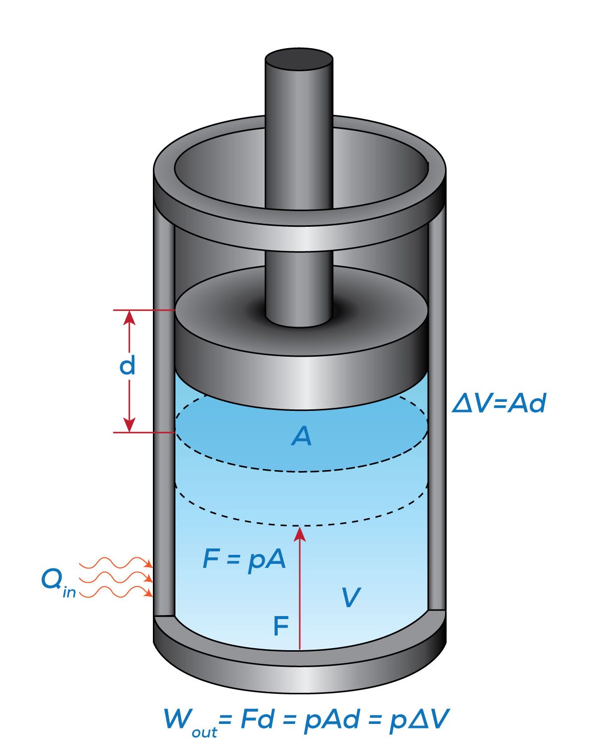
Let us consider a piston-cylinder device, as illustrated in Figure 4.3.2. The gas in the cylinder exerts an upward force, [latex]F=PA[/latex], where [latex]P[/latex] is the gas pressure, and [latex]A[/latex] is the cross-sectional area of the piston. Upon receiving heat, the gas will tend to expand, pushing the piston up. We will assume the expansion process is quasi-equilibrium, and the piston moves up an infinitesimal distance [latex]d[/latex]. The boundary work done by the gas to the surroundings in this infinitesimal process is [latex]dW=Fd=(PA)d=P(Ad)=P\Delta \mathbb{V}[/latex]; therefore, the total boundary work between two states in a process can be written as

[latex]{}_{1}W_{2}= \displaystyle\int_{1}^{2}{Pd\mathbb{V}\ }[/latex]

where

[latex]P[/latex]: pressure, in kPa or Pa

[latex]\mathbb{V}[/latex]: volume, in m³

[latex]{}_{1}W_{2}[/latex]: boundary work, in kJ or J

Specific boundary work refers to the boundary work done by a unit mass of a substance. It can be written as

[latex]{}_{1}w_{2}=\displaystyle\int_{1}^{2}{Pdv\ }[/latex]

where

[latex]P[/latex]: pressure, in kPa or Pa

[latex]v[/latex]: specific volume, in m³/kg

[latex]{}_{1}w_{2}[/latex]: specific boundary work, in kJ/kg or J/kg

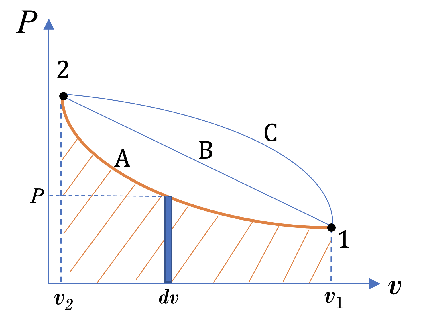
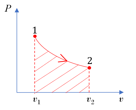
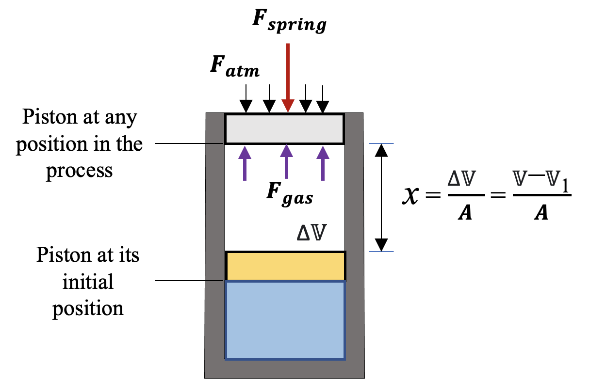
Boundary work caused by the expansion of gas in a piston cylinder device — **Figure 4.3.2** Boundary work caused by the expansion of gas in a piston-cylinder device

From the integral equations for [latex]{}_{1}W_{2}[/latex] and [latex]{}_{1}w_{2}[/latex], we can tell that the boundary work and specific boundary work between any two states in a process can be illustrated graphically as the area under the process curve in the [latex]P-\mathbb{V}[/latex] and [latex]P-v[/latex] diagrams, respectively. For example, the shaded area in Figure 4.3.3 represents the specific boundary work between states 1 and 2 in the compression process A. The three compression processes, A, B, and C in Figure 4.3.3 have different specific boundary work because of their different paths. By comparing the areas under the process curves, we can tell that process A has the smallest specific boundary work and process C has the largest specific boundary work.

Figure 4.3.3 demonstrates that the boundary work and specific boundary work in a quasi-equilibrium process are path functions; they depend on the initial and final states as well as the process path. Boundary work can be defined as positive or negative. Here is a common sign convention: the boundary work in an expansion process is positive. This is because the change of volume in an expansion process is positive. Likewise, the boundary work in a compression process is negative.

P-v diagram showing the area under the p-v curve as the boundary work — **Figure 4.3.3** P-v diagram showing the specific boundary work as the shaded area under the P-v curve

Example 1

Consider a rigid sealed tank of a volume of 0.3 m³ containing nitrogen at 10^oC and 150 kPa. The tank is heated until the temperature of the nitrogen reaches 50^oC. Treat nitrogen as an ideal gas.

Sketch the process on a [latex]P-\mathbb{V}[/latex] diagram
Calculate the boundary work in this process
Calculate the change in internal energy in this process

Solution

1. [latex]P-\mathbb{V}[/latex] diagram

**Figure 4.3.e1** Isochoric process in a rigid sealed tank

2. The boundary work is zero because the volume of nitrogen remains constant in the process.

[latex]{}_{1}W_{2}=\displaystyle \int_{1}^{2}{Pd\mathbb{V}\ }=0[/latex]

3. Change in internal energy in the process

From Table G1:

R=0.2968 kJ/kgK and C_v= 0.743 kJ/kgK

The mass of nitrogen:

[latex]\because P\mathbb{V} = mRT[/latex]

[latex]\therefore m = \dfrac{P\mathbb{V}}{RT} = \dfrac{150 \times 0.3}{0.2968 \times (273.15 + 10)} = 0.5355 \ \rm{kg}[/latex]

The change in internal energy:

[latex]\begin{align*} \Delta U &= m \Delta u =mC_v\left(T_2-T_1\right) \\&= 0.5355 \times 0.743 \times (50-10) = 15.9 \ \rm{kJ} \end{align*}[/latex]

Nitrogen absorbs 15.9 kJ of heat in this process.

Example 2

Consider 0.2 kg of ammonia in a reciprocating compressor (piston-cylinder device) undergoing an isobaric expansion. The initial and final temperatures of the ammonia are 0^oC and 30^oC, respectively. The pressure remains 100 kPa in the process.

Sketch the process on a [latex]P-v[/latex] diagram
Calculate the boundary work in this process
Calculate the change in internal energy in this process

Solution:

1. [latex]P-v[/latex] diagram

**Figure 4.3.e2** An isobaric expansion process in the superheated vapour region

2. Boundary work

From Table B2: for the initial state 1 at T = 0^oC, P = 100 kPa,

[latex]v_1 = 1.31365 \ \rm{m^3/kg}[/latex] [latex]u_1 = 1504.29 \ \rm{kJ/kg}[/latex]

For the final state 2 at T = 30^oC, P = 100 kPa,

[latex]v_2 = 1.46562 \ \rm{m^3/kg}[/latex] [latex]u_2 = 1554.1 \ \rm{kJ/kg}[/latex]

Graphically, the specific boundary work is the shaded rectangular area under the process line in the P – [latex]v[/latex] diagram.

[latex]\begin{align*} {}_{1}W_{2} &=m{}_{1}w_{2} = m\displaystyle\int_{1}^{2}{Pdv} = mP(v_2 - v_1) \\&= 0.2 \times 100 \times (1.46562 - 1.31365) = 3.0394 \ \rm{kJ} \end{align*}[/latex]

3. Change in internal energy

[latex]\begin{align*} \Delta U &= m \Delta u = m(u_2 - u_1) \\&= 0.2 \times (1554.1 -1504.29)= 9.962 \ \rm{kJ} \end{align*}[/latex]

Example 3

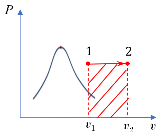
Consider air undergoing an isothermal expansion. The initial and final pressures of the air are 200 kPa and 100 kPa respectively. The temperature of the air remains 50^oC in the process. Treat air as an ideal gas.

Sketch the process on a [latex]P-v[/latex] diagram
Calculate the specific boundary work in this process
Calculate the change in specific internal energy in this process

Solution:

1. [latex]P-v[/latex] diagram

**Figure 4.3.e3** Isothermal expansion process

2. Specific Boundary work

From Table G1: R = 0.287 kJ/kgK for air. The ideal gas, air, undergoes an isothermal process.

[latex]\because Pv = RT[/latex]

[latex]\therefore P=\dfrac{RT}{v}[/latex] and [latex]\dfrac{v_2}{v_1} = \dfrac{P_1}{P_2}[/latex]

[latex]\begin{align*} {}_{1}W_{2}&=\displaystyle \int_{1}^{2}{Pdv} = \int_{1}^{2}{\dfrac{RT}{v }dv} \\&= RT\displaystyle\int_{1}^{2}{\dfrac{1}{v }dv} = RT ln\dfrac{v_2}{v_1} = RTln\dfrac{P_1}{P_2} \\&= 0.287 \times (273.15 + 50)ln\dfrac{200}{100} = 64.285 \ \rm{kJ} \end{align*}[/latex]

3. The process is isothermal; therefore, the temperature remains constant and the change in internal energy is zero.

[latex]\Delta u =C_v\left(T_2-T_1\right)=0[/latex]

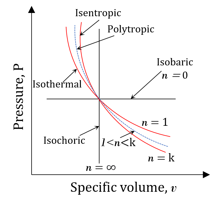
4.3.2 Polytropic process and its boundary work

A polytropic process refers to any quasi-equilibrium thermodynamic process, which can be described with the following mathematical expression.

[latex]P\mathbb{V}^n= \rm{constant}[/latex] or [latex]Pv^n= \rm{constant}[/latex]

where

[latex]P[/latex]: pressure, in kPa or Pa

[latex]\mathbb{V}[/latex]: volume, in m³

[latex]v[/latex]: specific volume, in m³/kg

[latex]n[/latex]: polytropic exponent, dimensionless

By adjusting [latex]n[/latex] to different values, the above two simple expressions can be used to represent the relations of pressure-volume or pressure-specific volume of various processes that are encountered in real thermal systems, including the isobaric, isochoric, and isothermal processes. Table 4.3.1 lists the polytropic exponents corresponding to an ideal gas undergoing an isobaric, isochoric, and isothermal process, respectively.

Table 4.3.1 Ideal gas equation of state expressed in polytropic relations
Process	Polytropic exponent	Ideal gas equation of state	Polytropic relation
Isobaric	[latex]n=0[/latex]	[latex]P= \rm{constant}[/latex]	[latex]Pv^0= \rm{constant}[/latex]
Isothermal	[latex]n=1[/latex]	[latex]\because T= \rm{constant}[/latex] and [latex]Pv=RT[/latex] [latex]\therefore Pv= \rm{constant}[/latex]	[latex]Pv^1= \rm{constant}[/latex]
Isochoric	[latex]n=\infty[/latex]	[latex]v= \rm{constant}[/latex]	[latex]Pv^\infty= \rm{constant}[/latex]

Figure 4.3.4 shows different polytropic processes of an ideal gas. In many actual thermodynamic processes, the polytropic exponents are typically in the range of [latex]1 \lt n \lt k[/latex], where [latex]k=\displaystyle\frac{C_p}{C_v}[/latex]. [latex]C_p[/latex] and [latex]C_v[/latex] are the constant-pressure and constant-volume specific heats, respectively.

P-v diagram showing different processes of an ideal gas — **Figure 4.3.4** Different processes of an ideal gas

The boundary work and corresponding specific boundary work in a polytropic process can be calculated by using the following equations. Detailed derivations are left for the readers to practice.

The following expressions are valid for both real and ideal gases.

If [latex]n \neq 1[/latex],

[latex]{}_{1}W_{2}=\displaystyle\frac{{P}_\mathbf{2}\mathbb{V}_\mathbf{2}-{P}_\mathbf{1}\mathbb{V}_\mathbf{1}}{1-n}\\[/latex]

[latex]\ {}_{1}w_{2}=\displaystyle\frac{{P}_\mathbf{2}{v}_\mathbf{2}-{P}_\mathbf{1}{v}_\mathbf{1}}{1-n}\\[/latex]

If [latex]\ n=1,[/latex]

[latex]{}_{1}W_{2}={P}_\mathbf{1}\mathbb{V}_\mathbf{1}{ln}{\displaystyle\frac{\mathbb{V}_\mathbf{2}}{\mathbb{V}_\mathbf{1}}}={P}_\mathbf{2}\mathbb{V}_\mathbf{2}{ln}{\displaystyle\frac{\mathbb{V}_\mathbf{2}}{\mathbb{V}_\mathbf{1}}}\\ [/latex]

[latex]{}_{1}W_{2}={P}_\mathbf{1}\mathbb{V}_\mathbf{1}{ln}{\displaystyle\frac{{P}_\mathbf{1}}{{P}_\mathbf{2}}}={P}_\mathbf{2}\mathbb{V}_\mathbf{2}{ln}{\displaystyle\frac{{P}_\mathbf{1}}{{P}_\mathbf{2}}}\\ [/latex]

[latex]\ {}_{1}w_{2}={P}_\mathbf{1}{v}_\mathbf{1}{ln}{\displaystyle\frac{{v}_\mathbf{2}}{{v}_\mathbf{1}}}={P}_\mathbf{2}{v}_\mathbf{2}{ln}{\displaystyle\frac{{v}_\mathbf{2}}{{v}_\mathbf{1}}}\\[/latex]

[latex]\ {}_{1}w_{2}={P}_\mathbf{1}{v}_\mathbf{1}{ln}{\displaystyle\frac{{P}_\mathbf{1}}{{P}_\mathbf{2}}}={P}_\mathbf{2}{v}_\mathbf{2}{ln}{\displaystyle\frac{{P}_\mathbf{1}}{{P}_\mathbf{2}}}\\[/latex]

The following two expressions are valid only for ideal gases in an isothermal process ([latex]\ n=1[/latex]).

If [latex]\ n=1,[/latex]

[latex]\ {}_{1}W_{2}={{mRT}}{ln}{\displaystyle\frac{\mathbb{V}_\mathbf{2}}{\mathbb{V}_\mathbf{1}}}={{mRT}}{ln}{\displaystyle\frac{{P}_\mathbf{1}}{{P}_\mathbf{2}}}\\ [/latex]

[latex]\ {}_{1}w_{2}={{RT}}{ln}{\displaystyle\frac{{v}_\mathbf{2}}{{v}_\mathbf{1}}}={{RT}}{ln}{\displaystyle\frac{{P}_\mathbf{1}}{{P}_\mathbf{2}}}\\[/latex]

where

[latex]{}_{1}W_{2}[/latex]: boundary work, in kJ or J

[latex]{}_{1}w_{2}[/latex]: specific boundary work, in kJ/kg or J/kg

[latex]P[/latex]: pressure, in kPa or Pa

[latex]\mathbb{V}[/latex]: volume, in m³

[latex]v[/latex]: specific volume, in m³/kg

[latex]T[/latex]: absolute temperature, in K

[latex]R[/latex]: gas constant, in kJ/kgK or J/kgK

[latex]m[/latex]: mass, in kg

Example 4

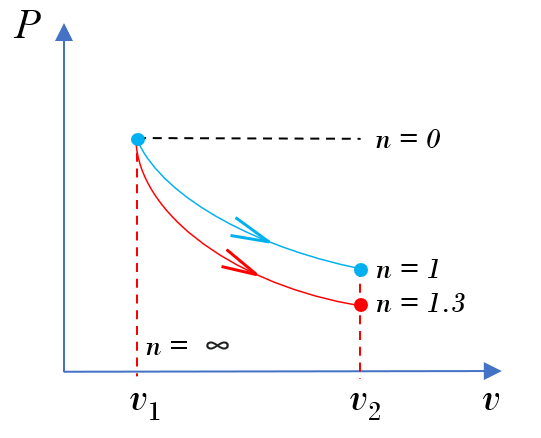
Consider an ideal gas undergoing a polytropic process. At the initial state: P₁=200 kPa, v₁=0.05 m³/kg. At the final state: v₂=0.1 m³/kg. For n=1.3 and n=1,

Sketch the two processes on a [latex]P-v[/latex] diagram. Which process has a larger specific boundary work?
Calculate the specific boundary work and verify your answer to the question in part 1.

Solution:

1. [latex]P-v[/latex] diagram

From the [latex]P - v[/latex] diagram, the area under the process line for [latex]n = 1[/latex] is greater than that for [latex]n = 1.3[/latex]; therefore, the isothermal process with [latex]n = 1[/latex] has a larger specific boundary work.

**Figure 4.3.e4** Polytropic processes of an ideal gas illustrated on the P-v diagram

2. For [latex]n=1.3[/latex], find the final pressure [latex]P_2[/latex] first.

[latex]\because P_1v_1^n = P_2v_2^n[/latex]

[latex]\therefore P_2 = P_1\left(\dfrac {v_1}{v_2}\right)^n = 200 \times \left(\dfrac{0.05}{0.1}\right)^{1.3} = 81.225 \ \rm{kPa}[/latex]

[latex]\begin{align*} {}_{1}W_{2} &= \dfrac{P_2v_2 - P_1v_1}{1-n} \\&= \dfrac{81.225 \times 0.1 - 200 \times 0.05}{1-1.3} = 6.258 \ \rm{kJ/kg} \end{align*}[/latex]

For [latex]n = 1[/latex], the process is isothermal; therefore,

[latex]\begin{align*} {}_{1}W_{2} &= P_1v_1ln \left(\dfrac{v_2}{v_1}\right) \\&= 200 \times 0.05 \times ln \dfrac{0.1}{0.05}= 6.931 \ \rm{kJ/kg} \end{align*}[/latex]

Compare the specific boundary work in these two processes, the isothermal process (n=1) has a larger specific boundary work than the polytropic process with n = 1.3. The calculation results are consistent with the observation from the [latex]P - v[/latex] diagram.

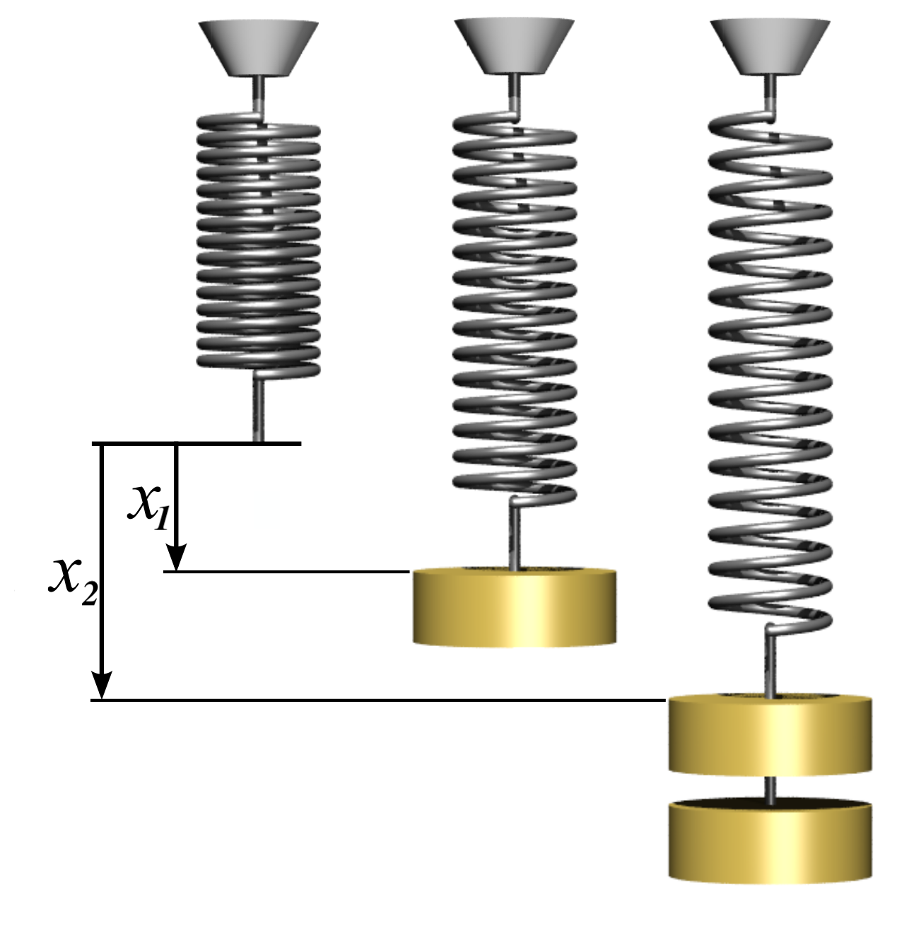
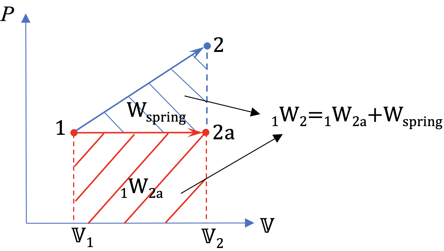
4.3.3 Spring work

Spring work is a form of mechanical energy required to compress or expand a spring to a certain distance, see Figure 4.3.5. Spring force and spring work can be expressed as follows:

[latex]F=Kx[/latex]

[latex]W_{spring}=\displaystyle\int_{1}^{2}{Fdx=}\displaystyle\frac{1}{2}K\left(x_2^2-x_1^2\right)[/latex]

where

[latex]F[/latex]: spring force, in kN or N

[latex]K[/latex]: spring constant, in kN/m or N/m

[latex]W_{spring}[/latex]: spring work, in kJ or J

[latex]x_1[/latex] and [latex]x_2[/latex]: initial and final displacements, in m, measured from the spring’s rest position.

Work done by the force acting on a spring causing expansion of the spring — **Figure 4.3.5** Work done by the spring force due to the displacement from the spring’s rest position.

Example 5

A linear spring with spring constant K=100 kN/m is mounted on a piston-cylinder device. At the initial state, the cylinder contains 0.15 m³ of gas at 100 kPa. The spring is uncompressed. The gas is then heated until its volume expands to 0.2 m³. The piston’s cross-sectional area is 0.1 m². Assume the piston is frictionless with negligible weight and the process is quasi-equilibrium,

1. Write an expression of the gas pressure as a function of the gas volume in this process
2. Sketch the process on a [latex]P-\mathbb{V}[/latex] diagram
3. Calculate the total work done by the gas during this expansion process
4. If the spring is not mounted on the piston, the gas in the cylinder will expand isobarically after being heated. To reach the same final volume, 0.2 m³, how much work must be done by the gas in the expansion process?
  
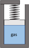
  Figure 4.3.e5 Piston-cylinder device with a spring loaded on top of the piston

Solution:

1. Analyze the forces acting on the piston, see below.

The piston is subject to three forces from the gas, the atmosphere and the spring. — **Figure 4.3.e6** Forces acting on the piston in static equilibrium

Three forces acting on the piston are in equilibrium.

[latex]\because\sum F = 0: F_{gas} = F_{spring} + F_{atm}[/latex]

[latex]\therefore P_{gas} A = Kx + P_{atm} A = K \dfrac{\mathbb{V} -\mathbb{V}_1}{A} + P_{atm} A[/latex]

[latex]\therefore P_{gas} = \dfrac{K(\mathbb{V}-\mathbb{V}_1)}{A^2} + P_{atm}[/latex]

At the initial state: [latex]P_{gas} = 100 \ \rm{kPa}, \mathbb{V}= \mathbb{V}_1[/latex]. Substitute the two values,

[latex]\because 100 = \dfrac{K(\mathbb{V}-\mathbb{V}_1)}{A^2} + P_{atm}[/latex]

[latex]\therefore P_{atm} = 100 \ \rm{kPa}[/latex]

with K =100 kN/m, A = 0.1 m², P_atm = 100 kPa and [latex]\mathbb{V}_1[/latex]= 0.15 m³, the gas pressure can be expressed as a function of the gas volume.

[latex]\because P_{gas} = \dfrac{100(\mathbb{V}-0.15)}{0.1^2} + 100[/latex]

[latex]\therefore P_{gas} = 10^4 \mathbb{V} -1400[/latex]

where gas pressure is in kPa and [latex]\mathbb{V}[/latex] is in m³.

2. [latex]P-\mathbb{V}[/latex] diagram

From part 1, P_gas is a linear function of volume [latex]\mathbb{V}[/latex].

P-V diagram of the process from the initial to the final states — **Figure 4.3.e7** P-V diagram showing the process from the initial to the final states

3. During the expansion process, the gas has to overcome the resistance from the springand. At the same time, the gas pressure and volume increase until the gas reaches the final state. The total work done by the gas is the shaded area of the trapezoid in the [latex]P-\mathbb{V}[/latex] diagram.

At the final state, [latex]\mathbb{V}_2= 0.2 \ m^3[/latex]; therefore,

[latex]P_{gas,2}= 10^4 \times 0.2 -1400 = 600 \ \rm{kPa}[/latex]

The total work done by the gas is

[latex]\begin {align*} {}_{1}W_{2} &= \dfrac{(P_{gas,2} + P_{gas,1})(\mathbb{V}_2 - \mathbb{V}_1)}{2} \\&= \dfrac{(600 + 100)(0.2 - 0.15)}{2} = 17.5 \ \rm{kJ} \end{align*}[/latex]

4. If the gas expands isobarically from [latex]\mathbb{V}_1[/latex] = 0.15 m³ to [latex]\mathbb{V}_2[/latex] = 0.2 m³, the work done by the gas will be

[latex]\begin {align*} {}_{1}W_{2a} &= P_{gas,1} (\mathbb{V}_2 - \mathbb{V}_1) \\&=100 \times (0.2 - 0.15) = 5 \ \rm{kJ} \end{align*}[/latex]

[latex]{}_{1}W_{2a}[/latex] is the shaded area of the rectangle. The difference between [latex]{}_{1}W_{2}[/latex] and [latex]{}_{1}W_{2a}[/latex] is the gas work used to overcome the resistance of the spring, as shown in the shaded area of the triangle.

[latex]W_{spring} = {}_{1}W_{2} - {}_{1}W_{2a} = 17.5 -5 = 12.5 \ \rm{kJ}[/latex]