5. The First Law of Thermodynamics for a Control Volume
5.3 Applications of the mass and energy conservation equations in steady flow devices
5.3.1 Turbines and compressors
Turbines and compressors are common energy conversion devices, in which the energy of a working fluid is converted to mechanical energy or vice versa. A typical turbine consists of rotor blades attached to a shaft, which is free to rotate. Figure 5.3.1 shows the main components of a hydraulic turbine. During the operation of a turbine, a working fluid (e.g., steam, gas, wind or water) flows continuously over a row of highly curved blades, creating a torque on the blades. In this process, the energy of the working fluid is converted to the mechanical energy of the rotating shaft. Consequently, the pressure and temperature of the fluid gradually decrease in the turbine. Figure 5.3.2 illustrates the energy conversion in a wind turbine. The wind energy is first converted to the mechanical energy of the shaft and gearbox, then converted to the electrical energy through the generator.
Compressors work in the opposite way to turbines. Compressors consume shaft power in order to increase the pressure of a working fluid, typically a gas. In a dynamic compressor, such as a centrifugal compressor, the increase of the gas pressure is achieved by forcing the gas into narrow passages formed by adjacent blades, which rotate around a shaft. Figure 5.3.3 shows a centrifugal compressor driven by an electric motor. In a reciprocating compressor, the increase of the gas pressure is achieved by the decrease of the gas volume as the piston, driven by a crank-shaft, compresses the gas. Figure 5.3.4 animates the expansion and compression processes in a reciprocating compressor. In both dynamic and reciprocating compressors, the mechanical energy of the rotating shaft or crank-shaft is converted to the energy stored in the fluid. As a result, the pressure of the fluid increases in the compressor.
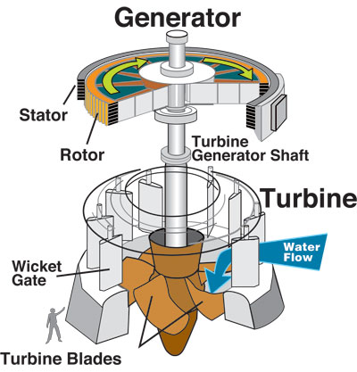
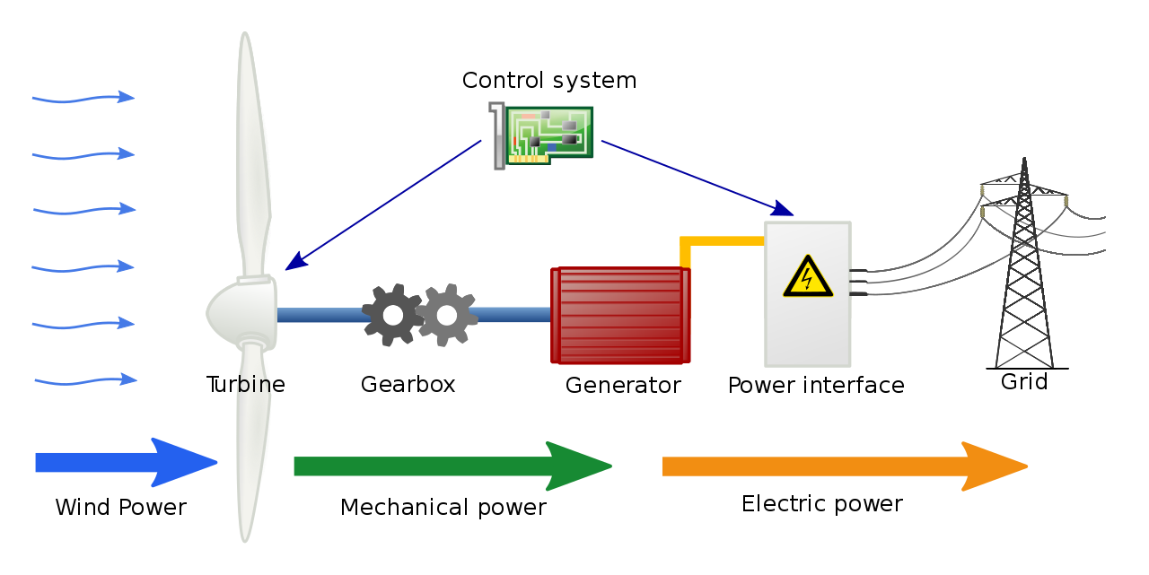
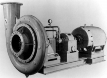
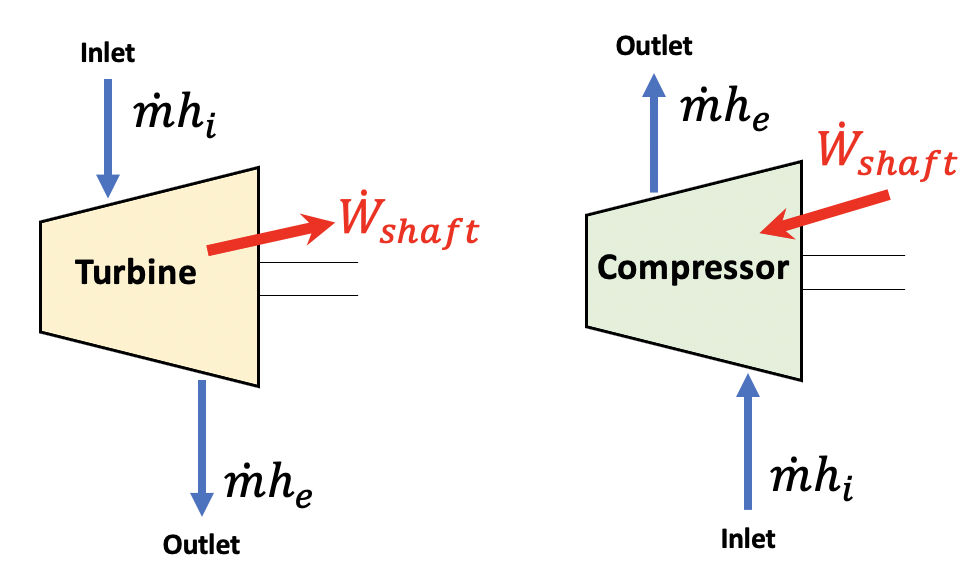
Figure 5.3.5 illustrates the flow of energy through a turbine and a compressor. A typical turbine or compressor has one inlet and one outlet. We may apply the following assumptions to typical turbines and compressors:
- The flow through a turbine or a compressor is steady.
- The turbine or compressor is well-insulated: [latex]\dot{Q}_{cv}=0[/latex]
- The changes in potential and kinetic energies are negligible compared to the change in enthalpy: [latex]\Delta PE = 0[/latex], [latex]\Delta KE = 0[/latex]
With these assumptions, the mass and energy conservation equations can be simplified as follows,
Turbine:
[latex]{\dot{m}}_i={\dot{m}}_e=\dot{m}[/latex]
[latex]{\dot{W}}_{shaft}=\dot{m}(h_i-h_e)[/latex]
Compressor:
[latex]{\dot{m}}_i={\dot{m}}_e=\dot{m}[/latex]
[latex]{\dot{W}}_{shaft}=\dot{m}(h_e-h_i)[/latex]
where
[latex]h[/latex]: specific enthalpy of the working fluid, in kJ/kg
[latex]\dot{m}[/latex]: mass flow rate of the working fluid through a turbine or compressor, in kg/m3
[latex]\dot{W}_{shaft}[/latex]: shaft power of the turbine or compressor, in kW
Subscripts, i and e, represent the inlet and exit of the turbine or compressor, respectively.
Example 1
The inlet and outlet conditions of an air compressor are P1=100 kPa, T1=20oC, and P2=300 kPa, respectively. The mass flow rate of air through this compressor is 0.015 kg/s. How much power input from the shaft is required to drive this compressor? Apply the following assumptions in your analysis: (1) the flow is steady with negligible changes in the kinetic and potential energies; (2) the compressor is well-insulated; (3) air is an ideal gas; and (4) the process is polytropic with n=1.35.
Solution:
Analysis: the shaft power of the compressor is proportional to the change in enthalpy of air in the compressor. Because air is treated as an ideal gas, the change in enthalpy can be calculated in terms of the change in temperature. Therefore, we need to find the temperature at the outlet of the compressor first.
Air is an ideal gas and the process is polytropic; therefore,
[latex]Pv = RT[/latex]
[latex]Pv^n = \rm{constant}[/latex]
Combine the above two equations and eliminate [latex]v[/latex],
[latex]P^{n-1} = \dfrac{R^n}{\rm{constant}} \times T^n[/latex]
Apply the above equation to the process between the inlet condition, state 1, and the outlet condition, state 2. Note that R is the gas constant of air,
[latex]\because \left(\dfrac{P_2}{P_1}\right)^{n-1} = \left(\dfrac{T_2}{T_1}\right)^{n}[/latex]
[latex]\begin{align*} \therefore T_2 &= T_1 \left(\dfrac{P_2}{P_1}\right)^{\dfrac{n-1}{n}} \\&= (273.15 + 20) \left(\dfrac{300}{100}\right)^{\dfrac{1.35-1}{1.35}} \\&= 389.75 \ \rm{K} = 116.6 \ {}^o \rm{C} \end{align*}[/latex]
From Table G1, Cp = 1.005 kJ/kgK for air. Apply the energy conservation equation to the compressor considering the first two assumptions in the question descriptions.
[latex]\begin{align*} {\dot{W}}_{shaft} &=\dot{m}(h_2-h_1) \\&=\dot{m}C_p(T_2 - T_1) \\&=0.015 \times 1.005\times (116.6 - 20) = 1.456 \ \rm{kW} \end{align*}[/latex]
The compressor consumes 1.456 kW of power when operating under the given conditions.
5.3.2 Throttling valves
Throttling valves are also called thermal expansion valves. They are used in vapour compression refrigeration systems to regulate the pressure in the evaporator as well as the superheat of the refrigerant flowing out of the evaporator. Throttling valves may be constructed as a porous plug, capillary tubes, or an adjustable valve such as an orifice, ball, or poppet valve. By restricting the refrigerant flow through the valve, a considerable pressure drop can be achieved. As the pressure of the refrigerant decreases, its corresponding saturation temperature decreases accordingly. Therefore, a phase change often occurs as the refrigerant passes through a throttling valve. Figure 5.3.6 shows a thermal expansion valve in a vapour compression refrigeration system. The following assumptions are commonly used for the analysis of the mass and energy conservation in a typical throttling valve.
- The flow through a throttling valve is steady.
- The flow through a throttling valve is fast enough so that the heat transfer between the refrigerant and its surroundings is negligible. Therefore, the flow is commonly treated as adiabatic: [latex]\dot{Q}_{cv}=0[/latex]
- No work exchange occurs between the refrigerant and its surroundings: [latex]\dot{W}_{cv}=0[/latex]
- The changes in potential and kinetic energies are negligible compared to the change in enthalpy: [latex]\Delta PE = 0[/latex], [latex]\Delta KE = 0[/latex]
Based on these assumptions, the mass and energy conservation equations in throttling valves can be written as
[latex]{\dot{m}}_i={\dot{m}}_e[/latex]
[latex]h_i=h_e[/latex]
where
[latex]h[/latex]: specific enthalpy of the refrigerant, in kJ/kg
[latex]\dot{m}[/latex]: mass flow rate of the refrigerant through a throttling valve, in kg/m3
Subscripts, i and e, represent the inlet and exit of the throttling valve, respectively.

Example 2
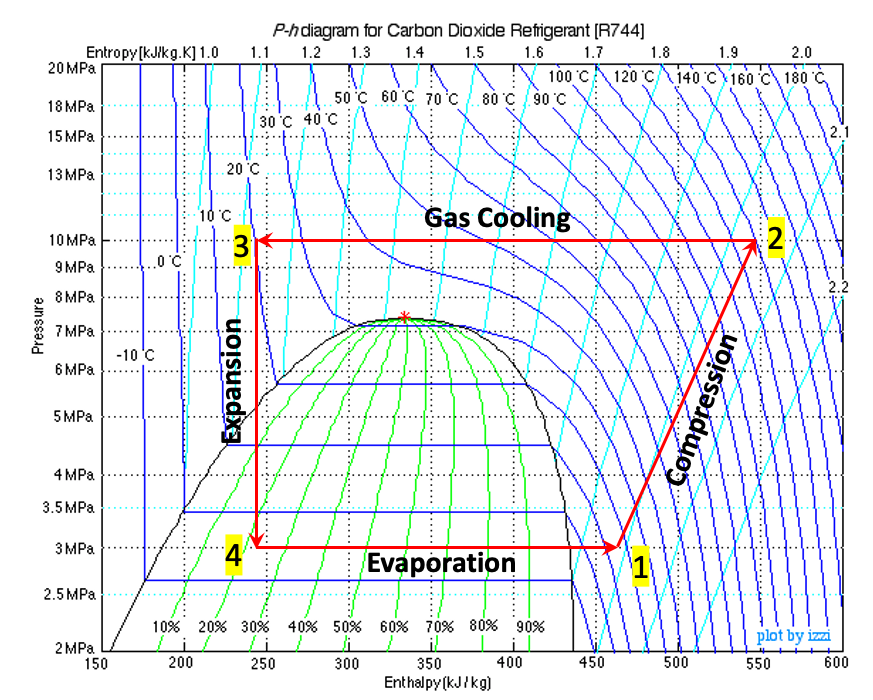
A simplified transcritical CO2 refrigeration cycle consists of four processes: compression (1[latex]\to[/latex]2), gas cooling (2[latex]\to[/latex]3), expansion (3[latex]\to[/latex]4), and evaporation (4[latex]\to[/latex]1), as shown in the [latex]P-h[/latex] diagram, Figure 5.3.e1. The CO2 gas enters the expansion valve at 10 MPa, 20oC (state 3) and is throttling to a pressure of 3 MPa (state 4). Determine the quality and temperature of CO2 at state 4.
Solution:
The specific enthalpy remains constant in the expansion process; therefore h3 = h4.
At state 3, P3 = 10 MPa, T3 = 20oC. From Table D2, h3 = 242.70 kJ/kg
At state 4, P4 = 3 MPa, h4 = h3 = 242.70 kJ/kg
From Table D1,
At T = -6oC , P = 2.96316 MPa, hf = 185.71 kJ/kg, hg = 433.79 kJ/kg
At T = -4oC, P = 3.13027 MPa, hf = 190.40 kJ/kg, hg = 432.95 kJ/kg
State 4 must be a two-phase mixture and its saturation temperature must be -6oC < T4 < -4oC. Use linear interpolation to determine the saturation temperature, T4, the specific enthalpy of the saturated liquid, hf,4, and the specific enthalpy of the saturated vapour, hg,4, of CO2 at P4 = 3 MPa.
[latex]\because \dfrac{T_{4}-(-6)}{(-4)-(-6)} =\dfrac{3-2.96316}{3.13027-2.96316}[/latex]
[latex]\therefore T_4 = -5.56 \ {}^\rm{o} \rm{C}[/latex]
[latex]\because\dfrac{h_{f,4}-185.71}{190.40-185.71}=\dfrac{h_{g,4}-433.79}{432.95-433.79} =\dfrac{3 - 2.96316 }{3.13027-2.96316}[/latex]
[latex]\therefore h_{f,4} = 186.74\ \rm{kJ/kg}[/latex] [latex]h_{g,4} = 433.60\ \rm{kJ/kg}[/latex]
The quality of the two phase mixture at state 4 is
[latex]x_4 = \dfrac{h_4 - h_{f,4}}{h_{g,4} - h_{f,4}} = \dfrac{242.70 - 186.74}{433.60 - 186.74} = 0.2267[/latex]
5.3.3 Nozzles and diffusers
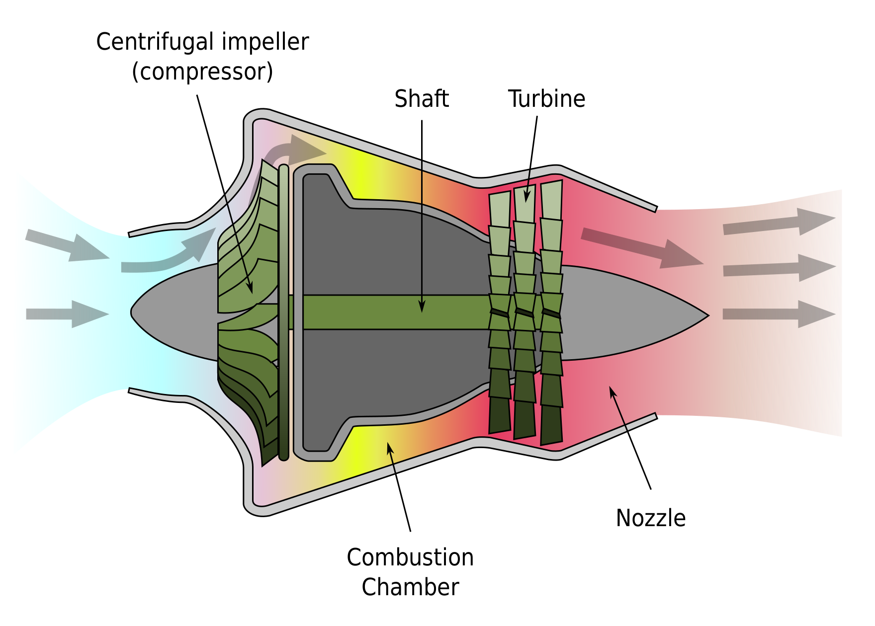
Nozzles and diffusers are devices used to accelerate or decelerate flow by gradually changing their cross-sectional areas. They are widely used in many engineering systems, such as piping systems, HVAC (heating, ventilating, and air conditioning) systems, and steam and gas engines. Figure 5.3.7 illustrates a turbojet engine, which consists of a centrifugal compressor, a combustion chamber, a turbine, and a nozzle section. The gas leaving the turbine is accelerated in the nozzle section, creating a high velocity jet, and thus a high thrust.
The flow in nozzles and diffusers can be subsonic or supersonic. In this book, we will only discuss subsonic nozzles and subsonic diffusers; thereafter, the terms "nozzle" and "diffuser" refer to subsonic nozzle and subsonic diffuser, respectively.
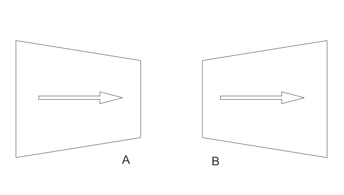
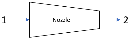
In a nozzle, the flow velocity increases and the pressure decreases as the cross-sectional area of the nozzle decreases. On the contrary, in a diffuser, the flow velocity decreases and the pressure increases as the cross-sectional area of the diffuser increases. Figure 5.3.8 shows a schematic of a nozzle and a diffuser. The following assumptions are commonly made when analyzing the mass and energy conservation in a typical nozzle or diffuser.
- The flow through a nozzle or diffuser is steady.
- The flow through a nozzle or diffuser is fast enough so that the heat transfer between the fluid and its surroundings is negligible. Therefore, the flow is commonly treated as adiabatic: [latex]\dot{Q}_{cv}=0[/latex]
- No work exchange occurs between the fluid and its surroundings: [latex]\dot{W}_{cv}=0[/latex]
- The change in potential energy is negligible compared to the changes in enthalpy and in kinetic energy: [latex]\Delta PE = 0[/latex]
With these assumptions, the mass and energy conservation equations in nozzles and diffusers can be written as
[latex]{\dot{m}}_i={\dot{m}}_e[/latex]
[latex]h_i+\displaystyle\frac{1}{2}V_i^2=h_e+\displaystyle\frac{1}{2}V_e^2[/latex]
where
[latex]h[/latex]: specific enthalpy of the fluid, in J/kg. Note: J/kg = m2/s2.
[latex]\dot{m}[/latex]: mass flow rate of the fluid through a nozzle or diffuser, in kg/m3
[latex]V[/latex]: velocity of the fluid, in m/s
Subscripts, i and e, represent the inlet and exit of the nozzle or diffuser, respectively.
Example 3
The inlet and outlet diameters of a hydrogen nozzle are 44 mm and 20 mm, respectively. Hydrogen enters the nozzle at -30oC, 5 bar, and 2 g/s, and exits the nozzle at 2 bar. Assuming the process is adiabatic and hydrogen is an ideal gas, what is the temperature and velocity of hydrogen at the nozzle outlet?
Solution:
Analysis: the energy conservation equation provides the relationship between the temperature, specific enthalpy, and velocity of the hydrogen. We will apply the mass and energy conservation equations to find the velocity and temperature at the nozzle outlet.
From Table G1: R = 4.124 kJ/kgK and Cp = 14.307 kJ/kgK for hydrogen.
Apply the mass flow rate and ideal gas law to the inlet of the nozzle:
[latex]\because \dot{m} = \rho_{1} V_{1}A_1[/latex] and [latex]P_1 = \rho_{1}RT_1[/latex]
[latex]\begin{align*} \therefore V_{1} &= \dfrac{\dot{m}_1RT_1}{P_{1}A_1} \\&= \dfrac{0.002 \times 4.124 \times (273.15 -30)}{500 \times \pi \times 0.022^2} = 2.638 \ \rm{m/s} \end{align*}[/latex]
Apply the mass conservation equation and the ideal gas law to the inlet and outlet of the nozzle:
[latex]\because \dot{m}_1 = \dot{m}_2[/latex]
[latex]\therefore \rho_{1} V_{1}A_1 = \rho_{2} V_{2}A_2[/latex]
and [latex]P_1 = \rho_{1}RT_1 \ , \ P_2 = \rho_{2}RT_2[/latex]
[latex]\begin{align*} \therefore V_2 &= V_1 \dfrac{A_{1}P_{1}T_{2}}{A_{2}P_{2}T_{1}} = V_1 \dfrac{P_{1}T_{2}}{P_{2}T_{1}} \times \left(\dfrac{D_1}{D_2}\right)^2 \\&=2.638 \times \dfrac{5 \times T_{2}}{2 \times T_{1}} \times \left(\dfrac{44}{20}\right)^2 = 31.92 \dfrac{T_2}{T_1} \end{align*}[/latex]
Apply the energy conservation equation to the inlet and outlet of the nozzle:
[latex]h_1+\displaystyle\frac{1}{2}V_1^2=h_2+\displaystyle\frac{1}{2}V_2^2[/latex]
and [latex]\Delta h = C_p(T_2-T_1)[/latex] for ideal gases
therefore,
[latex]C_{p}T_1+\displaystyle\frac{1}{2}V_1^2=C_{p}T_2+\displaystyle\frac{1}{2}V_2^2[/latex]
Substitute [latex]V_2 = 31.92 \dfrac{T_2}{T_1}[/latex] and rearrange
[latex]1 + \dfrac{V_1^2}{2C_{p}T_1} = \dfrac{T_2}{T_1} + \dfrac{1}{2C_{p}T_1}\left(31.92 \dfrac{T_2}{T_1}\right)^2[/latex]
Substitute V1 = 2.638 m/s, T1 =273.15 - 30 = 243.15 K, Cp = 14307 J/kgK into the above relation, and rearrange,
[latex]0.00014643 \left(\dfrac{T_2}{T_1}\right)^2 + \dfrac{T_2}{T_1} -1 =0[/latex]
[latex]\therefore \dfrac{T_2}{T_1} = 0.99985[/latex]
[latex]\therefore T_2 = 0.99985 \times 243.15 = 243.11\ K = -30.04\ {}^\rm{o} \rm{C}[/latex]
[latex]\therefore V_2 = 31.92\dfrac{T_2}{T_1} = 31.91 \ \rm{m/s}[/latex]
In this nozzle, the velocity increases significantly as the pressure decreases. The temperature remains almost constant.
Important note:
- The temperatures in the calculations must be in Kelvin because the ideal gas law is used to derive other equations.
- The constant-pressure specific heat must be in J/kgK to ensure the consistency of the units.
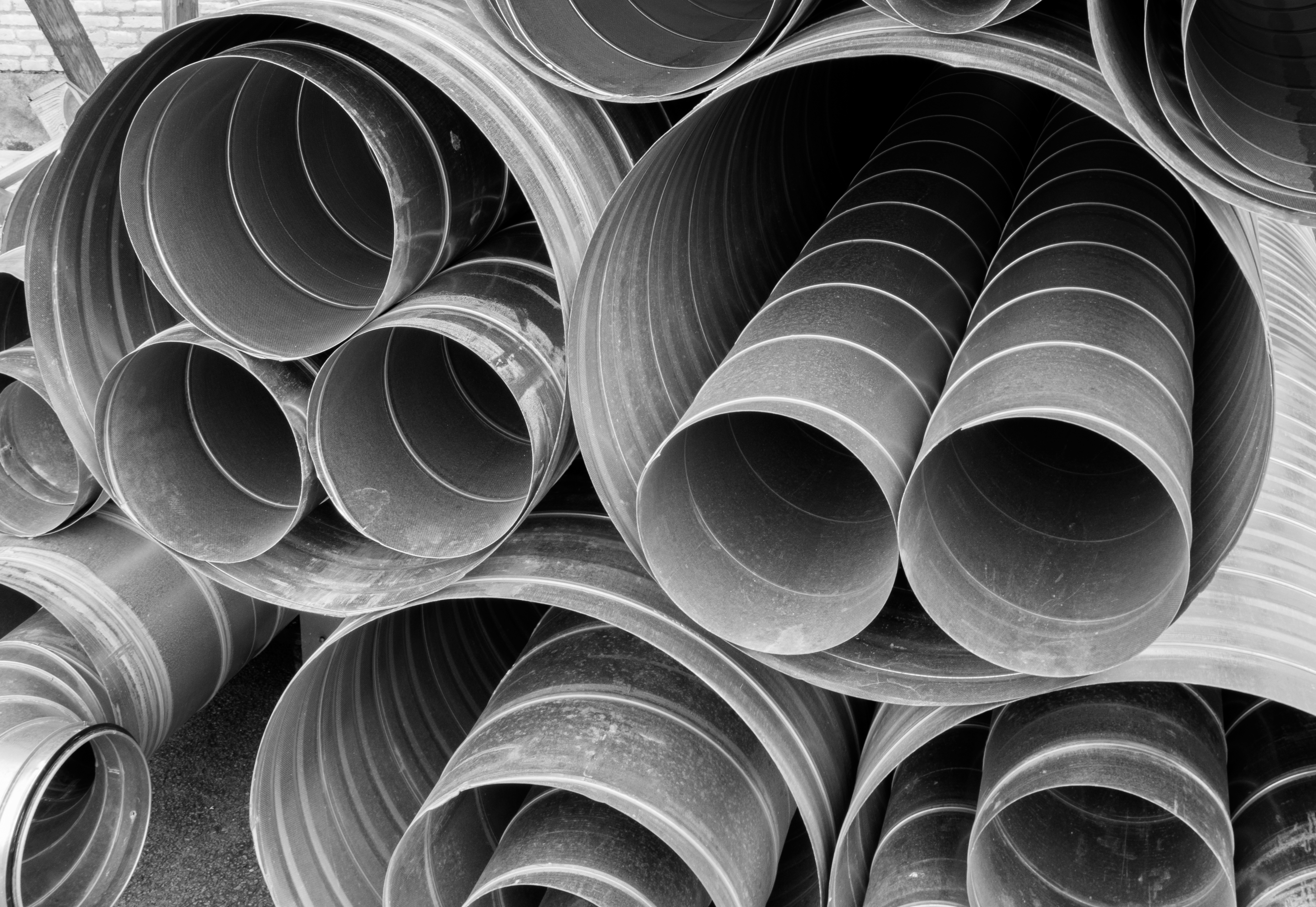
5.3.4 Ducts and pipes
Ducts and pipes are used to transport liquids and gases. Their configurations vary largely with applications; therefore, it is impractical to apply general assumptions to all ducts and pipes. Ducts and pipes may be analyzed specifically with the mass and energy conservation equations in Section 5.2.
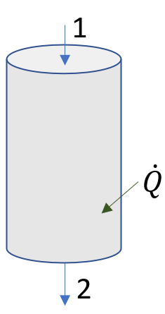
Example 4
Consider a vertical pipe section exposed to the ambient. The pipe has a constant diameter of 100 mm. Its inlet is 5 m above its outlet. Water at 10oC and 100 kPa enters the pipe at a velocity of 2 m/s, and exits at 12oC and 100 kPa. Assuming steady flow, what is the rate of heat transfer absorbed by the water in this pipe section?
Solution:
From Table A1, water is a compressed liquid at both inlet and outlet conditions, therefore,
[latex]v_1 \approx v_2 = v_f = 0.001 \ \rm{m^3/kg}[/latex]
[latex]\rho_1 \approx \rho_2 = \dfrac{1}{v_f }= 1000\ \rm{kg/m^3}[/latex]
Mass flow rate is
[latex]\dot{m} = \rho_{1} V_{1}A_1 = 1000 \times 2 \times \pi \times 0.05^2 = 15.7 \ \rm{kg/s}[/latex]
Apply the energy conservation equation to the pipe section
[latex]\dot{Q} + \dot{m}\left(h_1+\displaystyle\frac{1}{2}V_1^2+gz_1\right)=\dot{m}\left(h_2 + \displaystyle\frac{1}{2}V_2^2+gz_2\right)[/latex]
Since the diameter of the pipe section and the density of water remain constant in the pipe, the inlet and outlet velocity must be the same based on the mass conservation equation. From Table G2: Cp =4.181 kJ/kgK = 4181 J/kgK for water.
[latex]\because V_1= V_2[/latex]
[latex]\begin{align*} \therefore \dot{Q} &= \dot{m}(h_2 - h_1 + gz_2 - gz_1) \\&= \dot{m}Cp(T_2 - T_1) + \dot{m}g(z_2 - z_1) \\&= 15.7 \times 4181 \times (12-10) + 15.7 \times 9.81 \times (-5) \\&= 130580 \ \rm{W} = 130.6 \ \rm{kW} \end{align*}[/latex]
The water absorbs 130.6 kW of heat from the ambient.
Important note:
- The constant-pressure specific heat must be in J/kgK in the calculations to ensure the consistency of the units.
5.3.5 Mixing chambers
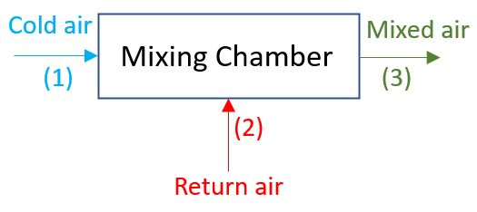
Mixing chambers are devices used to mix multiple streams of a fluid to achieve a desirable temperature or phase in the mixed flow. Figure 5.3.10 is a schematic of a mixing chamber in HVAC systems, where the outdoor fresh air mixes with the indoor return air in order to achieve a desirable air temperature and a targeted fresh air to return air ratio. The common assumptions for analyzing the mass and energy conservation in a mixing chamber are listed below:
- The flow through a mixing chamber is steady.
- No work exchange occurs between the mixing chamber and its surroundings: [latex]\dot{W}_{cv}=0[/latex]
- The changes in potential and kinetic energies are negligible: [latex]\Delta PE = 0[/latex], [latex]\Delta KE = 0[/latex]
- The pressure variation in a mixing chamber is usually negligible.
With these assumptions, the mass and energy conservation equations in mixing chambers can be written as
[latex]\sum{{\dot{m}}_i=\sum{\dot{m}}_e}[/latex]
[latex]{\dot{Q}}_{cv}+\sum{{\dot{m}}_ih_i=\sum{{\dot{m}}_eh_e}}[/latex]
where
[latex]h[/latex]: specific enthalpy of the fluid, in kJ/kg
[latex]\dot{m}[/latex]: mass flow rate, in kg/m3
[latex]{\dot{Q}}_{cv}[/latex]: rate of heat transfer entering the mixing chamber, in kW
Subscripts, i and e, represent the inlets and exits of the mixing chamber, respectively.
Example 5
Consider a well-insulated mixing chamber in an HVAC system, see Figure 5.3.10. The cold outdoor air at -10oC and 100 kPa mixes with the return air at 22oC and 100 kPa. The mass flow rates of the outdoor air and return air are 0.5 kg/s and 3 kg/s, respectively. Assume the flow is steady and the air is an ideal gas under the given conditions. What is the air temperature leaving the mixing chamber?
Solution:
Apply both mass and energy conservation equations to the mixing chamber:
[latex]\dot{m}_1 + \dot{m}_2 = \dot{m}_3[/latex]
[latex]{\dot{m}}_1h_1 +{\dot{m}}_2h_2 ={\dot{m}}_3h_3[/latex]
[latex]\Delta h = C_p \Delta T [/latex] (for ideal gases)
From the above three equations,
[latex]\begin{align*} T_3 &= \dfrac{\dot{m}_{1}T_2 + \dot{m}_{2}T_2}{\dot{m}_1 + \dot{m}_2} \\&= \dfrac{0.5 \times (-10) + 3 \times (22)}{0.5 + 3} = 17.43 \ {}^ \rm{o} \rm{C} \end{align*}[/latex]
The mixed air leaves the mixing chamber at a temperature of 17.43oC. In this calculation, the temperatures can be expressed either in oC or Kelvin as as long as the consistent units are used.
5.3.6 Heat exchangers
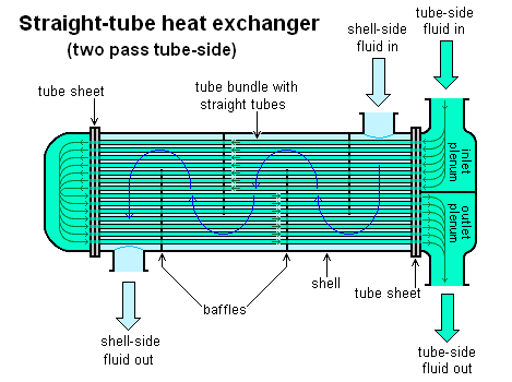
Heat exchangers are used to transfer heat between two flowing fluids. They can be found in many applications, such as HVAC systems, automotive systems, power generation plants, and chemical processing. Heat exchangers come in different types. For example, Figure 5.3.11 shows a tube-within-shell heat exchanger, where heat is transferred between the shell-side fluid and the tube-side fluid. The tube-within-shell heat exchanger is a typical indirect heat exchanger, in which the two fluids don’t mix during the heat transfer process.
Below are the common assumptions for analyzing the mass and energy conservation in an indirect heat exchanger:
- The flows through an indirect heat exchanger are steady.
- Each flow passage has only one inlet and one outlet.
- No work exchange occurs between the heat exchanger and its surroundings: [latex]\dot{W}_{cv}=0[/latex]
- The changes in potential and kinetic energies are negligible: [latex]\Delta PE = 0[/latex], [latex]\Delta KE = 0[/latex]
- The pressure variation in a heat exchanger is usually negligible.
With these assumptions, the mass and energy conservation equations for an indirect heat exchanger can be written as
[latex]{\dot{m}}_{i, hot}={\dot{m}}_{e, hot}[/latex]
[latex]{\dot{m}}_{i, cold}={\dot{m}}_{e, cold}[/latex]
[latex]{\dot{Q}}_{cv}+\sum{{\dot{m}}_ih_i=\sum{{\dot{m}}_eh_e}}[/latex]
where
[latex]h[/latex]: specific enthalpy of the fluid, in kJ/kg
[latex]\dot{m}[/latex]: mass flow rate, in kg/m3
[latex]{\dot{Q}}_{cv}[/latex]: rate of heat transfer entering the heat exchanger, in kW
Subscripts, i and e, represent the inlet and exit of the heat exchanger, respectively.
Subscripts, hot and cold, represent the hot and cold streams, respectively, through the heat exchanger.
It is important to note that, although the mass and energy conservation equations derived for mixing chambers and heat exchangers look very similar, there exists a major difference between these two devices. In a mixing chamber, all flow streams mix and exit as a single stream; therefore, both mass and energy conservation equations are applied to the entire mixing chamber consisting of all flow streams. On the contrary, in an indirect heat exchanger, the cold and hot streams do NOT mix; therefore, the mass conservation equation must be applied to each flow stream individually. The energy conservation equation may be applied to the entire heat exchanger or each flow stream individually.
Example 6
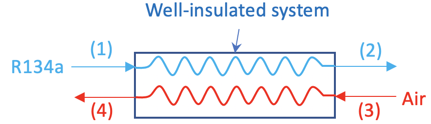
Consider the evaporator of a vapour compression refrigeration system using R134a as the working fluid. R134a enters the evaporator at -10oC with a quality of 0.1 and exits as a saturated vapour. Air enters the evaporator in a separate stream at 25oC and exits at 5oC. Assume (1) the evaporator is well-insulated; (2) the flow is steady; (3) the pressure remains constant in the evaporator; and (4) air is an ideal gas. What is the mass flow rate of air required in this system if the mass flow rate of R134a is 2 kg/s?
Solution:
Apply the mass conservation equations to the R134a and air streams, separately.
[latex]\dot{m}_1 = \dot{m}_2 = \dot{m}_{R134a}[/latex]
[latex]\dot{m}_3 = \dot{m}_4 = \dot{m}_{air}[/latex]
Apply the energy conservation equation to the evaporator.
[latex]\because\dot{m}_1 h_1 +\dot{m}_3 h_3 =\dot{m}_2 h_2 +\dot{m}_4 h_4[/latex]
[latex]\therefore \dot{m}_{air}(h_3 - h_4) = \dot{m}_{R134a}(h_2 - h_1)[/latex]
[latex]\therefore \dot{m}_{air} = \dot{m}_{R134a} \dfrac{(h_2 - h_1)}{(h_3 - h_4)}[/latex]
Find the specific enthalpies of R134a at states 1 and 2 using thermodynamic tables.
At state 1, T1 = -10oC, x= 0.1. From Table C1, hf = 186.70 kJ/kg, hg = 392.67 kJ/kg
[latex]\begin{align*} h_1 &= h_f + x(h_g - h_f) \\&= 186.70 + 0.1 \times (392.67 -186.70) = 207.297 \ \rm{kJ/kg} \end{align*}[/latex]
At state 2, R134a is a saturated vapour at T2 = -10oC; therefore,
[latex]h_2 = h_g = 392.67 \ \rm{kJ/kg}[/latex]
From Table G1, Cp,air = 1.005 kJ/kgK. Therefore,
[latex]\begin{align*} \dot{m}_{air} &= \dot{m}_{R134a} \dfrac{(h_2 - h_1)}{C_{p,air}(T_3 - T_4)} \\&= 2\times \dfrac{392.67 -207.297}{1.005 \times (25-5)} = 18.445 \ \rm{kg/s} \end{align*}[/latex]
The system requires an air supply at a rate of 18.445 kg/s.
Practice Problems
Practice Problems
Media Attributions
- Hydraulic turbine © U.S. Army Corps of Engineers is licensed under a Public Domain license
- Wind turbine schematic © Jalonsom is licensed under a CC BY-SA (Attribution ShareAlike) license
- Centrifugal compressor © UN document (USGOV) is licensed under a Public Domain license
- Reciprocating compressor © Birpat is licensed under a CC BY-SA (Attribution ShareAlike) license
- Thermal expansion valve © MasterTriangle12 is licensed under a CC BY-SA (Attribution ShareAlike) license
- P-h diagram for CO2 © Israel Urieli is licensed under a CC BY-SA (Attribution ShareAlike) license
- Turbojet © Original design: Emoscopes (talk)Vectorization: Tachymètre is licensed under a CC BY (Attribution) license
- Nozzle and diffuser © Nemuri is licensed under a CC BY-SA (Attribution ShareAlike) license
- HVAC pipes © W.carter is licensed under a Public Domain license
- Straight tube heat exchanger © H Padleckas is licensed under a CC BY-SA (Attribution ShareAlike) license
