6. Entropy and the Second Law of Thermodynamics
6.4 Carnot cycles
6.4.1 Irreversibilities
The Kelvin-Planck and Clausius statements of the second law indicate that for heat engines, [latex]\eta_{th}< 1[/latex], and for refrigerators and heat pumps, [latex]COP< \infty[/latex]. But can [latex]\eta_{th} \to 1[/latex] and [latex]COP \to \infty[/latex] in an ideal condition? How is an ideal process or cycle defined? What is the theoretical limit of [latex]\eta_{th}[/latex] or [latex]COP[/latex] in an ideal cycle? To answer these questions, we will first need to understand the concepts of reversible processes and irreversibilities.
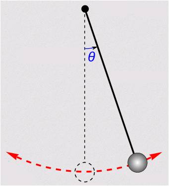
A reversible process is a process that can be reversed without leaving any change in either the system or its surroundings, which means both the system and its surroundings always return to their original states during a reversible process. A fictitious, frictionless pendulum can be treated as a reversible process, see Figure 6.4.1; it will never stop and always returns to its original state. However, in reality, friction always exists. A pendulum will gradually slow down and eventually stop.
Factors that render a process irreversible are called irreversibilities. Friction, unrestrained expansion, mixing of fluids, heat transfer through a finite temperature difference, electric resistance, inelastic deformation of solids, and chemical reactions are some examples of irreversibilities. All processes occurring in nature are irreversible due to the existence of irreversibilities. Some processes are more irreversible than others. A reversible process is commonly used as an idealized model to which an actual process can be compared. The efficiency of a reversible process is the theoretical limit that an actual, irreversible process can possibly achieve in a nearly ideal condition.
6.4.2 Carnot heat engine
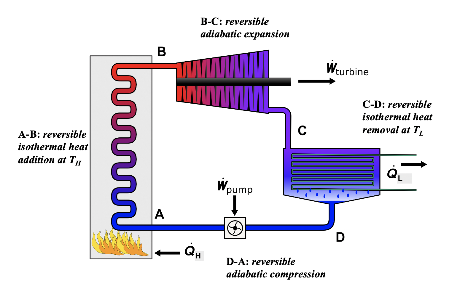
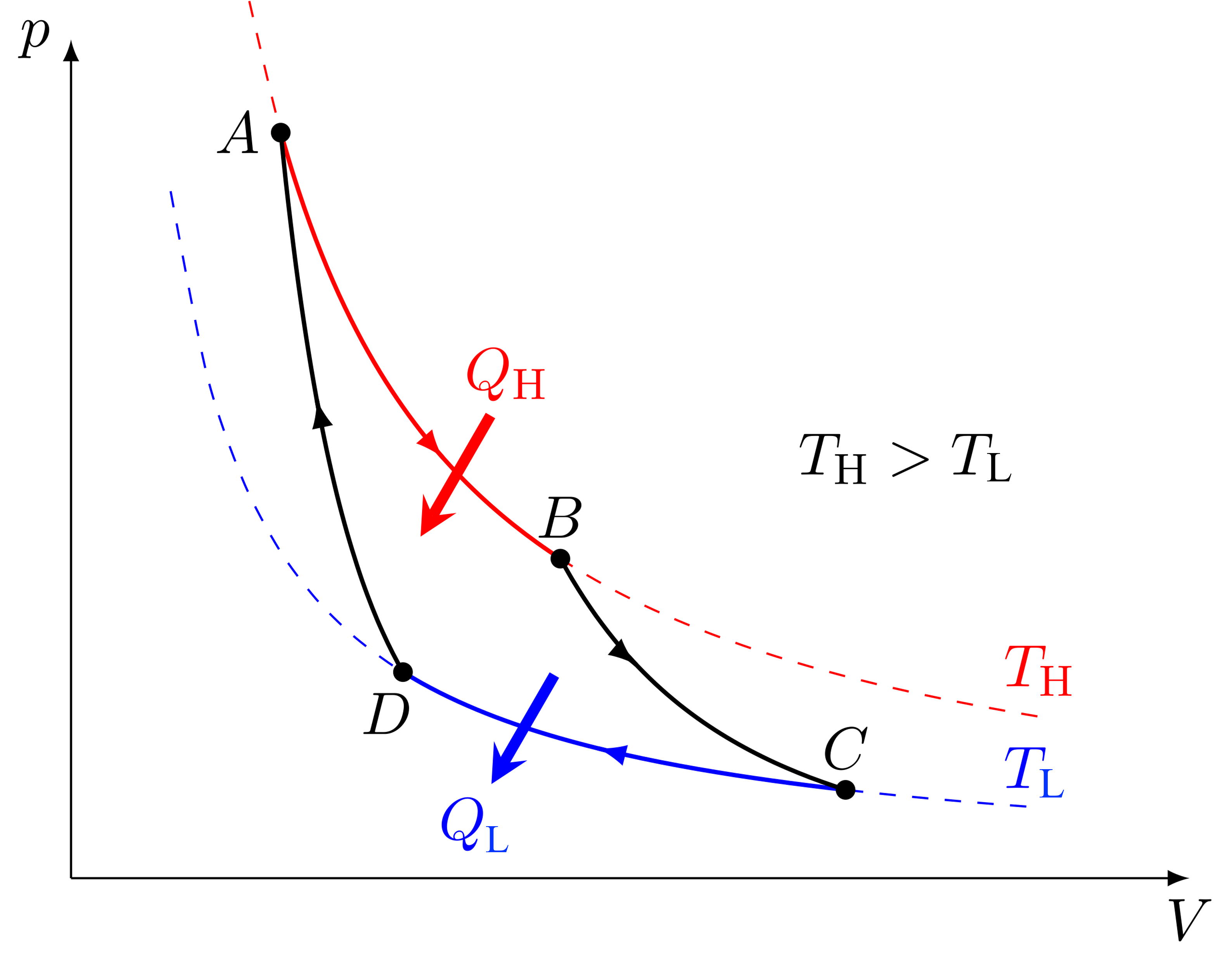
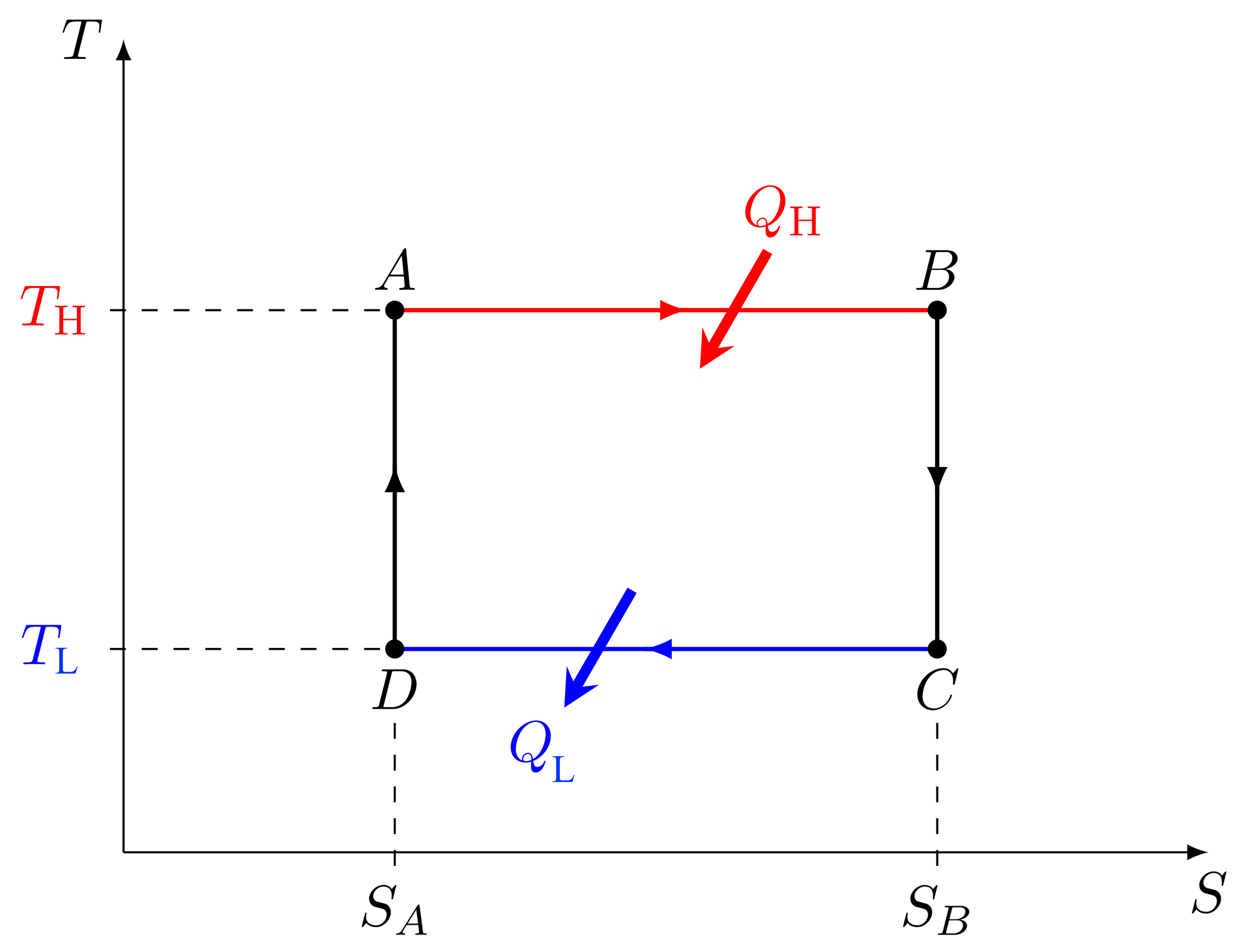
A Carnot heat engine is an idealized cycle, which consists of four reversible processes. Figures 6.4.2-6.4.4 show the schematic of a Carnot heat engine and its pressure-volume, [latex]P-\mathbb{V}[/latex], and temperature-entropy, [latex]T-S[/latex], diagrams. The cycle consists of the following four reversible processes:
- Process A[latex]\to[/latex]B: a reversible isothermal heat addition process of [latex]Q_H[/latex] from a heat source at constant temperature [latex]T_H[/latex].
- Process B[latex]\to[/latex]C: a reversible adiabatic expansion process, during which the temperature drops from [latex]T_H[/latex] to [latex]T_L[/latex].
- Process C[latex]\to[/latex]D: a reversible isothermal heat removal process of [latex]Q_L[/latex] from a heat sink at constant temperature [latex]T_L[/latex].
- Process D[latex]\to[/latex]A: a reversible adiabatic compression process, in which the temperature increases from [latex]T_L[/latex] to [latex]T_H[/latex].
Because the Carnot heat engine cycle is an ideal cycle consisting of only reversible processes, it produces the maximum power output and has the maximum thermal efficiency among all heat engines operating between the same heat source at [latex]T_H[/latex] and the same heat sink at [latex]T_L[/latex]. The thermal efficiency of a Carnot heat engine can be expressed as
[latex]\eta_{th,\ rev}= 1-\left(\displaystyle\frac{Q_L}{Q_H}\right)_{rev} = 1-\displaystyle\frac{T_L}{T_H}[/latex]
where
[latex]T_H[/latex]: absolute temperature of the heat source, in Kelvin
[latex]T_L[/latex]: absolute temperature of the heat sink, in Kelvin
[latex]Q_H[/latex]: heat supplied by the heat source to the Carnot heat engine, in kJ
[latex]Q_L[/latex]: heat rejected from the Carnot heat engine to the heat sink, in kJ
[latex]\eta_{th,\ rev}[/latex]: thermal efficiency of the Carnot heat engine, dimensionless
The thermodynamic temperature scale, or absolute temperature scale is defined so that [latex]\left(\displaystyle\frac{Q_L}{Q_H}\right)_{rev} = \displaystyle\frac{T_L}{T_H}[/latex].
In summary, the thermal efficiency of an actual heat engine is always less than that of the Carnot heat engine. It is impossible for any heat engine to achieve a better performance than the Carnot heat engine operating between the same heat source at [latex]T_H[/latex] and the same heat sink at [latex]T_L[/latex].
- Irreversible, actual heat engine: [latex]\eta_{th}<\eta_{th,\ rev}[/latex]
- Carnot heat engine: [latex]\eta_{th}=\eta_{th,\ rev}[/latex]
- Impossible device: [latex]\eta_{th}>\eta_{th,\ rev}[/latex]
For a heat engine operating between a heat source at [latex]T_H[/latex] and a heat sink at [latex]T_L[/latex], either increasing [latex]T_H[/latex] or decreasing [latex]T_L[/latex] can improve its thermal efficiency. In practice, much effort is made to increase the temperature of the heat source [latex]T_H[/latex] within the material limits because the temperature of the heat sink [latex]T_L[/latex] is usually constrained by the ambient temperature. In many large steam power plants, the temperature of the inlet steam (heat source) is in the range of 300~600oC (573~873 K) in order to improve the thermal efficiency of the heat engines.
Example 1
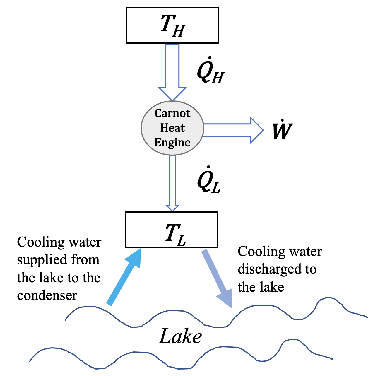
Consider a proposal to build a 500-MW steam power plant operating on a Rankine cycle by a lake. The steam generated by the boiler is at 250°C. The condenser is to be cooled by the lake water at a flow rate of 20 m3/s. As the cooling water will be discharged to the lake, the design team needs to evaluate its impact on the local aquatic ecosystem. Assume the cooling water supplied from the lake to the condenser is at a constant temperature of 18°C.
- If the cycle were reversible (Carnot cycle), what is the thermal efficiency of the power plant? Estimate the temperature rise of the discharge water to the lake.
- If the cycle were reversible (Carnot cycle), and the steam temperature increases to 300oC, how would the thermal efficiency of the power plant change?
- The above two scenarios are ideal Carnot cycles. In fact, the projected thermal efficiency of the actual cycle is about 35%. Estimate the temperature rise of the discharge water to the lake in this case.
Solution:
1. The power plant is assumed to operate on a Carnot cycle between a heat source at the steam temperature of TH = 250°C and a heat sink at the cooling water temperature of TL = 18°C. The thermal efficiency of the Carnot cycle is
[latex]\eta_{th,rev} = 1 - \dfrac{T_L}{T_H} = 1 - \dfrac{273.15 + 18}{273.15 + 250} = 0.443[/latex]
[latex]\eta_{th,rev} = \dfrac{\dot{W}}{\dot{Q}_H}[/latex] and [latex]\dot{Q}_H = \dot{Q}_L + \dot{W}[/latex]
Therefore, the heat rejected to the discharge water to the lake is
[latex]\begin{align*} \dot{Q}_L &= \dot{W}\left(\dfrac{1}{\eta_{th,rev}} - 1 \right) \\&= 500\left(\dfrac{1}{0.443} - 1 \right) = 627.48 \ \rm{MW} \end{align*}[/latex]
From Table G2, Cp = 4.181 kJ/kgK for water, and the density of water is [latex]\rho = 1000 \ \rm{kg/m^3}[/latex]; therefore,
[latex]\because \dot{Q}_{L} = \dot{m}C_p \Delta T = \rho \dot{\mathbb{V}}C_p \Delta T[/latex]
[latex]\therefore \Delta T = \dfrac{\dot{Q}_{L}}{\rho \dot{\mathbb{V}}C_p} = \dfrac{627.48 \times 10^3}{1000 \times 20 \times 4.181} = 7.5 \ {}^ \rm{o} \rm{C}[/latex]
2. For a Carnot cycle with TH = 300°C and TL = 18°C,
[latex]\eta_{th,rev} = 1 - \dfrac{T_L}{T_H} = 1 - \dfrac{273.15 + 18}{273.15 + 300} = 0.492[/latex]
Comment:
Compare the two Carnot cycles, increasing the heat source temperature TH can increase the thermal efficiency of the cycle. Similarly, decreasing the heat sink temperature TL can also increase the thermal efficiency of the cycle.
3. The thermal efficiency of an actual cycle is always less than that of the Carnot cycle operating between the same heat source and heat sink. If the projected thermal efficiency of the actual cycle is 35%, then the heat absorbed by the discharge water will be
[latex]\begin{align*} \dot{Q}_{L} &= \dot{W}\left(\dfrac{1}{\eta_{th}} - 1\right) \\& = 500 \times \left(\dfrac{1}{0.35} - 1\right) = 928.57 \ \rm{MW} \end{align*}[/latex]
The temperature rise of the discharge water will be
[latex]\Delta T = \dfrac{\dot{Q}_{L}}{\rho \dot{\mathbb{V}}C_p} = \dfrac{928.57}{1000 \times 20 \times \times 4.181} = 11.1 \ {}^ \rm{o} \rm{C}[/latex]
Comment:
The actual cycle will cause a much higher temperature rise in the discharge water than the Carnot cycle due to the existence of the irreversibilities. A large amount of heat rejection to the lake could have a negative impact on the aquatic life and should be monitored closely.
6.4.3 Carnot refrigerator and Carnot heat pump
If the four processes, compression, evaporation, expansion and condensation, in a vapour-compression refrigeration system are all reversible, the cycle is reversible and is called the Carnot refrigeration cycle. A refrigerator or a heat pump operating in such a cycle is called a Carnot refrigerator or a Carnot heat pump.
Among all refrigerators (or heat pumps) operating between the same heat source at [latex]T_H[/latex] and the same heat sink at [latex]T_L[/latex], the Carnot refrigerator (or heat pump) consumes the least amount of power, thus achieving the highest coefficient of performance, [latex]{COP}_{R,\ rev}[/latex] or [latex]{COP}_{HP,\ rev}[/latex], as expressed below:
- Carnot refrigerator: [latex]{COP}_{R,\ rev}=\displaystyle\frac{T_L}{T_H-T_L}=\frac{1}{T_H/T_L-1}[/latex]
- Carnot heat pump: [latex]{COP}_{HP,\ rev}=\displaystyle\frac{T_H}{T_H-T_L}=\displaystyle\frac{1}{{1-T}_L/T_H}[/latex]
where
[latex]{COP}_{R,\ rev}[/latex]: coefficient of performance of a Carnot refrigerator, dimensionless
[latex]{COP}_{HP,\ rev}[/latex]: coefficient of performance of a Carnot heat pump, dimensionless
[latex]T_H[/latex]: absolute temperature of the heat source, in Kelvin
[latex]T_L[/latex]: absolute temperature of the heat sink, in Kelvin
Example 2
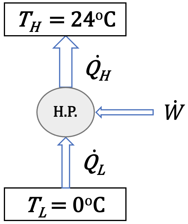
A heat pump provides 20 kW of heating to a house in winter. The house must be maintained at 24oC. If the COP of the heat pump is 5.5, and the outdoor temperature is 0oC, answer the following questions.
- How much power is required to drive the heat pump? Compare the power consumption of this heat pump and an electric resistance heater providing the same amount of heating to the house.
- If the cycle were a Carnot cycle, what would the power consumption be?
- If the outdoor temperature decreases, will the COP of the heat pump increase, remain the same, or decrease?
Solution:
1. The heat pump provides 20 kW of heating to the house; therefore, [latex]\dot{Q}_{H} = 20 \ \rm{kW}[/latex]
[latex]\because \; COP_{HP} = \dfrac{\dot{Q}_{H}}{\dot{W}}= 5.5[/latex]
[latex]\therefore \; \dot{W} = \dfrac{\dot{Q}_{H}}{{COP}_{HP}} = \dfrac{20}{5.5} = 3.636 \ \rm{kW}[/latex]
If an electric resistance heater is used to provide 20 kW of heating to the house, the electric resistance heater will consume 20 kW of electric power, assuming the efficiency of the heater is 100%. Therefore,
[latex]\Delta \dot{W} = 20 - 3.636 = 16.364 \ \rm{kW}[/latex]
Compare the power consumption of the heat pump and electric heater, using heat pump will save 16.354 kW of power.
2. If the cycle were a Carnot cycle,
[latex]\begin{align*} COP_{HP,rev} &= \dfrac{T_{H}}{T_{H} - T_{L}} \\&= \dfrac{273.15 + 24}{(273.15 + 24) - (273.15 + 0)}= 12.38 \end{align*}[/latex]
[latex]\because \; COP_{HP,rev} = \dfrac{\dot{Q}_H}{\dot{W}_{rev}}[/latex]
[latex]\therefore \; \dot{W}_{rev} = \dfrac{\dot{Q}_{H}}{COP_{HP,rev}} = \dfrac{20}{12.38} = 1.615 \ \rm{kW}[/latex]
The actual cycle achieves a much smaller COP and consumes a much greater power than the Carnot cycle due to the irreversibilities.
3. Since [latex]COP_{HP,rev} = \dfrac{T_{H}}{T_{H} - T_{L}} = \dfrac{1}{1 - T_L/T_H}[/latex]
As [latex]T_H[/latex] is a constant room temperature, [latex]COP_{HP, rev}[/latex] will decrease if the outdoor temperature [latex]T_L[/latex] decreases. Because the Carnot cycle always has the maximum COP compared to any real cycle operating between the same heat source and heat sink, the COP of a real heat pump will also decrease if the outdoor temperature decreases; therefore, heat pumps are preferably used in mild winter conditions.
Practice Problems
Media Attributions
- Frictionless pendulum © Chetvornoderivative work: Py4nf is licensed under a CC0 (Creative Commons Zero) license
- Carnot heat engine © Andrew Ainsworth is licensed under a CC BY-SA (Attribution ShareAlike) license
- Carnot heat engine: P-v diagram © Cristian Quinzacara is licensed under a CC BY-SA (Attribution ShareAlike) license
- Carnot heat engine: T-s diagram © Cristian Quinzacara is licensed under a CC BY-SA (Attribution ShareAlike) license
A reversible process refers to a process that can be reversed without leaving any changes in either the system or its surroundings. In a reversible process, both the system and its surroundings can always return to their original states.
Irreversibilities refer to factors that render a process irreversible.
