10.2.1 The Linear Regression Model and the Line of Best Fit

You might have noticed that there was no uncertainty of any kind in the Example 10.2 about the assignment requirements and mark in the previous section. The line in that case represented a deterministic relationship — x fully determined y (i.e., x fully explained the variability of y) — hence all the observation were on the line itself.

As such, this was not a typical situation and this was not a typical regression line. In reality, in statistical inference we deal with probabilistic associations, where the regression line does not capture all observations in itself but their general (on average) trend. That is, in a usual regression model situation, some observations will be above the line and some below it; thus some observations would be underestimated and others would be overestimated because the line serves as a prediction (an expectation, a summary, a trend) of the association. And as we know by now, predictions/estimations always contain a level of uncertainty.

Specifically, we cannot expect that a single independent variable x will explain away all variability in a dependent variable y; there will always be some unexplained (by the regression model) variability left. Figure 10.2 illustrates.

Figure 10.2 Assignment Mark as a Function of Completed Requirements (With Variance)

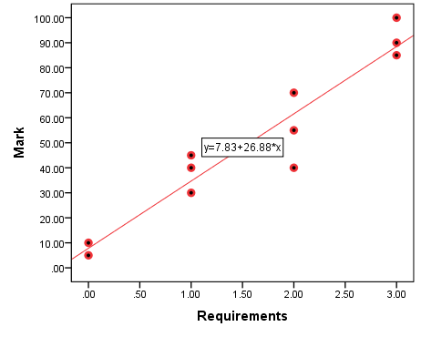
In Figure 10.2 I have added seven more observations to the case we had in Figure 10.1 in the previous section, this time allowing for additional variability in the assignment marks: no longer is it enough to know the number of requirements completed to predict the assignment grade. (Imagine that the professor has started evaluating the completed requirements substantively, not just counting them: in this case while the number of requirements is still essential for the grade, something else^[1] also affects the final assignment mark.)

An actual regression model accommodates the uncertainty inherent in estimation through two interrelated concepts, error of prediction (a.k.a. statistical error) and residuals.

The error of prediction reflects the difference between the observations and the predicted values we would have if we had data about the population. That is, if we imagined a line of best fit of the population^[2], α+βx, the difference between our observations and that line would be:

= error of prediction^[3]

That is, we need to include the error term in the regression model:

Considering that we pretty much never have information about the population, however, we can restate the sample regression model like this:

where a is the estimated α, b is the estimated β, and e is the estimated ε, with all estimations based on sample data. Note that e here is called the residual, and it is not only the estimation of the unobservable error of prediction, but also simply the difference between an observation and its predicted value:

= residual

Since a+bx is the regression line, or the prediction, it also stands for the predicted (estimated values), which we can, as usual, denote . Then, since

,

we also have

or, again, that the residuals are the difference between the observations and their predicted values.

With this, we come at a full circle and the reason for all the notation and protracted explanations above (and here you thought I was subjecting you to all these equations without a purpose): in a graph, the residuals are simply the distance between the observations and the regression line. (In Figure 10.2 this is the empty space — the shortest distance — between an observation and the regression line.)

A comprehensive treatment of the residuals (through a full-blown analysis of variance) is beyond the scope of this book but they do help us understand the nature of the regression line and of the logic of regression in general. You see, the regression line is called a line of best fit precisely because it minimizes the residuals — it is created in such a way as to minimize the residuals (and therefore the error of prediction) and fit the data/observations as best as possible. Visually, this will mean that the line is drawn to pass as close as possible to all the observations.

In fact, linear regression is also called OLS regression, which stands for ordinary least squares. The least squares concept comes from the fact that to minimize the distances of the observations to the prediction line, we need to first square them before adding them together^[4] — just like we needed to do that in the calculation of the variance and the sum of squares (or the distances would cancel each other out)^[5].

But how do we ensure that the regression line minimizes the residuals? The next section explains.