Chapter 5 The Normal Distribution and Some Basics of Probability
5.2.5 The Real Use of z-Values
Recall from Section 5.1.2 (here: https://pressbooks.bccampus.ca/simplestats/chapter/5-1-2-the-z-value/) that any value/score can be converted into a z-value, which tells us how far the value is from the mean in terms of standard deviations. Now that we know the normal curve has a bell shape reflecting probabilities (the higher the curve at any point, the bigger the probability), any point on the horizontal axis can be seen as a z-value associated with a specific probability — or rather, the probability below and the probability above the z-value.
You can find the z-values’ probabilities listed in a Normal Distribution Table, e.g., this one: https://www.mathsisfun.com/data/standard-normal-distribution-table.html. Note that since the normal distribution is symmetric (i.e., the left side, below the mean, is exactly the same as the right side, above the mean), such tables usually only list probabilities between the mean and the z-score and above the z-score. This needs to be taken into account when calculating probabilities.[1]
Alternatively, online normal distribution calculators like this one http://onlinestatbook.com/2/calculators/normal_dist.html give you the option to specify which probability you need calculated based on a specific mean and standard deviations.
Let’s take an example to see how this works.
Example 5.4 Hockey Player Heights
According to Hockey Graphs (REFERENCE https://hockey-graphs.com/2015/02/19/nhl-player-size-from-1917-18-to-2014-15-a-brief-look/), the average height of players in the National Hockey League is about 185 cm, with a standard deviation of about 5.3 cm[2].
What is the probability that a new recruit (to your team of choice) will be taller than 185 cm? (Suspend disbelief and assume the recruit is randomly selected; i.e., his height (or skill) has absolutely no bearing on his selection.)
This one is easy: 185 cm is the mean, so the probability of a particular height being above the mean is 50 percent (equal to the probability of a height being below the mean). (For a visual, refer to Fig. 5.6 (B) in the previous section.)
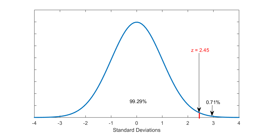
So let’s complicate matters further: What is the probability of the new recruit being taller than 198 cm?
To find it, we first need to convert the value into a z-score:
![\[z=\frac{x_i - \mu}{\sigma}=\frac{198-185}{5.3}=\frac{13}{5.3}=2.45\]](https://pressbooks.bccampus.ca/simplestats/wp-content/ql-cache/quicklatex.com-9cfeac3d235fd10a6dd1bf5cc5a3fd44_l3.png "Rendered by QuickLaTeX.com")
where of course xi is the original value, μ is the mean, and σ is the standard deviation.
Then, using a normal distribution table (e.g., the one linked above, https://www.mathsisfun.com/data/standard-normal-distribution-table.html[3]), we find that the probability for a height to be above z=2.45 (i.e., above 198 cm) corresponds to 0.71 percent, or less than 1 percent. (Of course, if you’re curious, you’ll also know that the probability of a new recruit to be shorter than 198 cm is (100-0.71=) 99.29 percent.)
You can see the correspondence between the two graphs below in Fig. 5.7, one showing the height values and the other the z-scores. The area in which we are interested is beyond/above 198 cm, i.e., beyond/above z=2.45.
Figure 5.7 (A) The Area Beyond 198 cm
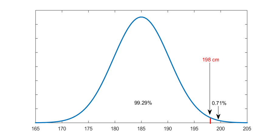
Figure 5.7 (B) The Area Beyond z = 2.45
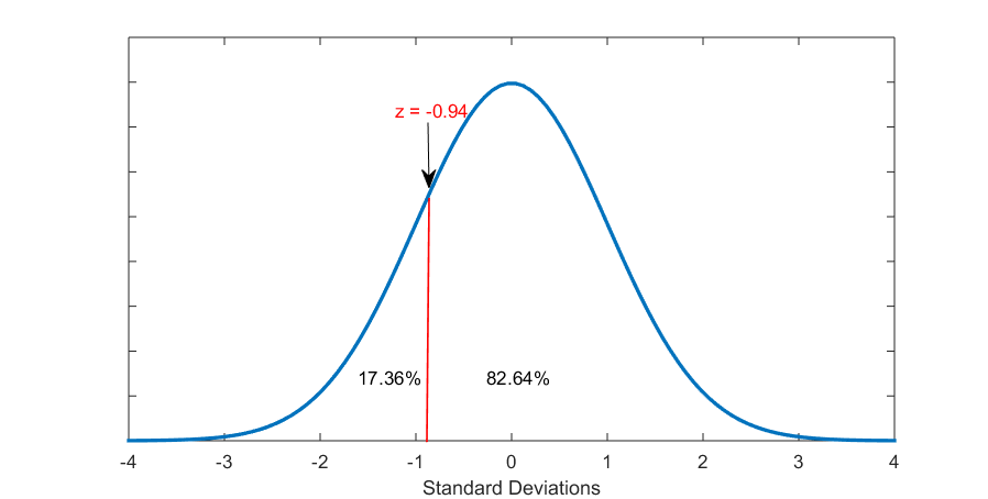
We can also ask the probability of a team recruit being shorter than 180 cm. Then:
![\[z=\frac{x_i - \mu}{\sigma}=\frac{180-185}{5.3}=\frac{-5}{5.3}=-0.94\]](https://pressbooks.bccampus.ca/simplestats/wp-content/ql-cache/quicklatex.com-db366ece88fdf30c1848fb952b48878e_l3.png "Rendered by QuickLaTeX.com")
Checking the normal distribution table, we find that the probability up to/below z=-0.94 is 17.36 percent. Thus we have found that the probability of a recruit to be shorter than 180 cm is 17.36 percent. (Alternatively, we also know that the probability of a recruit being taller than 180 cm is (100-17.36=) 82.65 percent.) Again, see the graphs in Fig. 5.8 below.
Figure 5.8 (A) The Area Up To 180 cm
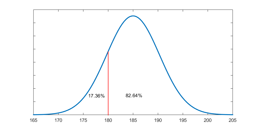
Figure 5.8 (B) The Area Up To z = -0.94
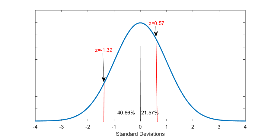
Finally, let’s try finding the probability of a new recruit being between 178 cm and 188 cm. In this case we need to find two z-scores, and add the probabilities between each of the z-scores and the mean (i.e., above the lower score up to the mean, and below the higher score down to the mean).
![\[z=\frac{x_i - \mu}{\sigma}=\frac{178-185}{5.3}=\frac{-7}{5.3}=-1.32\]](https://pressbooks.bccampus.ca/simplestats/wp-content/ql-cache/quicklatex.com-9d3c12300bd8733f6c5cc8c68d32345a_l3.png "Rendered by QuickLaTeX.com")
![\[z=\frac{x_i - \mu}{\sigma}=\frac{188-185}{5.3}=\frac{3}{5.3}=0.57\]](https://pressbooks.bccampus.ca/simplestats/wp-content/ql-cache/quicklatex.com-d39445c0a34c7f0eda942f282bfb2aa2_l3.png "Rendered by QuickLaTeX.com")
Using a normal distribution table we find that the probability between z=-1.32 and the mean is 40.66 percent. The probability between the mean and z=0.57 is 21.57 percent. Thus, the probability that a new recruit’s height will be between 178 cm and 188 cm is (40.66+21.57=) 62.23 percent. See Fig. 5.9 below.
Figure 5.9 (A) The Area Between 178 cm and 188 cm (Or Rather Between 178 cm and 185 cm and Between 185 cm and 188 cm)
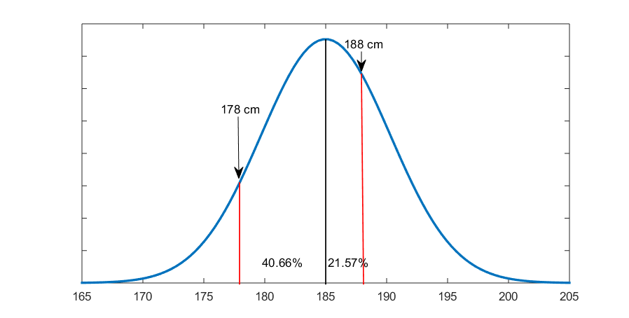
Figure 5.9 (B) The Area Between z = -1.32 and z = 0.57 (Or Rather Between z = -1.32 and 0 and Between 0 and z = 0.57)
Time to practice on your own!
Do It! 5.8 Test Scores
Imagine you learn that the average score on some test you’ve taken is 110 with a standard deviation 8. You still don’t know your score, so you’ll try to estimate some probabilities. What is the probability that you have more than 130? What about more than 95? Below 87? Between 90 and 115? Feel free to use the normal distribution table linked above. (Hint: Drawing out the normal curve centered on 110 helps.)
(Answers: z=2.5, 0.62%; z=-1.88, 96.99%; z=-2.88, 0.2%; z=-2.5 and z=0.63, 49.38% + 23.57%= 72.95%)
Now, with the concepts of probabilities and the normal distribution under your belt, you are finally ready to delve into statistical inference. Unfortunately for you, another theoretical chapter looms on the horizon, next. Grit your teeth and bear it, for the payoff (once we get to actually applying the theory in practice) is well worth it.