Chapter 5 The Normal Distribution and Some Basics of Probability
5.1.1 Properties of the Normal Curve
Recall that we describe a distribution via three things: its shape, its central tendency measures, and its measures of dispersion. The perfect (i.e., theoretical) normal distribution thus has three defining features.
First, the normal curve is bell-shaped and perfectly symmetric (i.e., if you bisect it in the middle, the left side will be identical to the right side).[1]
Second, the normal curve is centered on the mean, which also happens to be equal to its median and mode. That is, for the normal curve all measures of central tendency fall on the same value.
Third, the normal curve’s standard deviation tell us what percentage of observations fall within a specific distance from the mean. When we have a normal curve, the area below the curve contains 100 percent of all observations. Then, 68 percent of all observations fall within 1 standard deviation from the mean[2]; 95 percent of observations fall within about 2 standard deviations from the mean[3]; and 99 percent of observations fall within about 3 standard deviations from the mean[4]. Fig. 5.3 illustrates.
Figure 5.3 Normal Curve with Standard Deviations
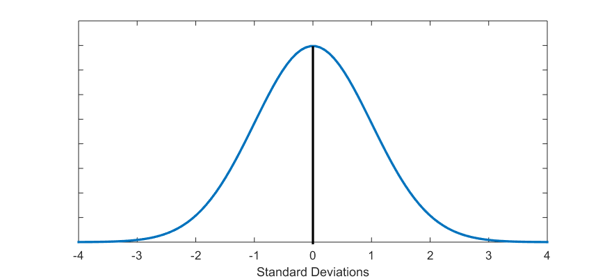
If you imagine Fig. 5.3 interposed on top of an approximately distributed variable’s histogram, you can see what percentage of observations will fall within 1, 2, and 3 standard deviations from the mean. (Obviously, the mean is at 0, since the normal curve is centered on the midway point of the curve, and is neither below nor above itself, i.e., “the mean is 0 standard deviations away from the mean”, as awkward as it sounds.)
Let’s make sure this makes sense to you in applied terms, through the example below.
Example 5.1 Normally Distributed Test Scores (Hypothetical Data)
Imagine your statistics class has taken a test. The average test score is 65 with a standard deviation of 10 and the following scores distribution. (You can imagine a histogram whose many bars follow the curve in the three Fig. 5.4 below.)
Figure 5.4 (A) Test Scores within 1 Standard Deviation
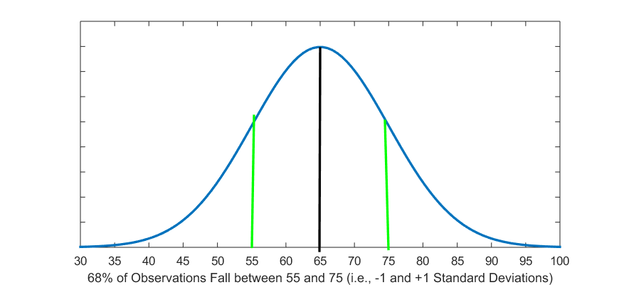
Figure 5.4 (B) Test Scores within About 2 Standard Deviations
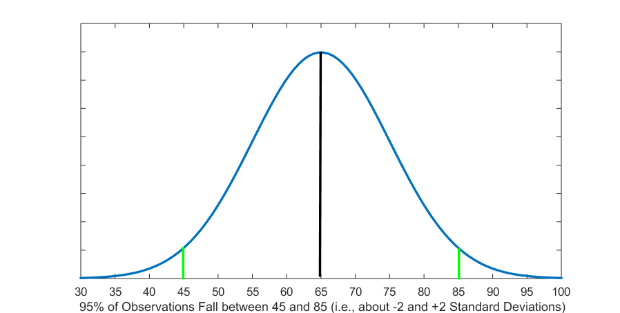
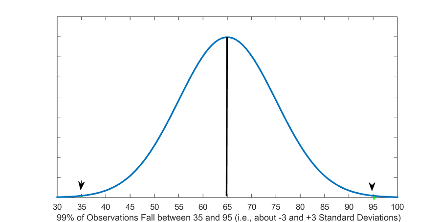
Figure 5.4 (B) Test Scores within About 3 Standard Deviations
Given the properties of the normal curve, we now know that 68 percent of students in the class scored between 55 and 75 (i.e., between -1 and +1 standard deviations from the mean, and since the standard deviation is 10, then  and
and  ). We also know that 95 percent of students scored approximately between 45 and 85 (i.e., between about -2 and +2 standard deviations from the mean, or
  and
and  ). Finally, we know that 99 percent of students (almost everyone!) scored approximately between 35 and 95 (i.e., between -3 and +3 standard deviations from the mean, or 65-3(10)=65-30=35
 65+3(10)=65+30=95$).
As is typical of normal distributions, the majority of scores (68 percent) are clustered in the middle (within -1 and +1 standard deviations) around the mean; the remaining 32 percent are split between the “tails” of the distribution, with about 16 percent in each “tail” beyond -1 and beyond +1 standard deviation from the mean. Only 5 percent of test scores are as far away as -2 and +2 standard deviations from the mean, with just 2.5 percent at the tips of each of the “tails”. And at the very, very far ends of the “tails”, beyond the -3 and +3 standard deviations from the mean, you have 1 percent split between them, so a minuscule 0.5 percent of students has a score below 35 and another 0.5 percent has a score above 95.
These features of the normal distribution (symmetrical, centered on the mean/median/mode, measured in standard deviations from the mean) make it very useful to work with. Simultaneously, now you can begin to see why the standard deviation is the most popular measure of dispersion, due to its unique relationship with the normal curve.
Can we find more uses of the normal distribution? Read on to find out.
- It's also asymptotic to the horizontal axis line, i.e., it gets as close to it as possible in the "tails" without ever touching it. More on this after you learn about probabilities. ↵
- Given the symmetry, this means 34 percent fall within -1 standard deviation below and 34 percent fall within +1 standard deviation above the mean. ↵
- That is, 47.5 percent fall within about -2 standard deviations below the mean and 47.5 fall within about +2 standard deviations above the mean. ↵
- That is, 49.5 percent fall within about -3 standard deviations below the mean and 49.5 percent fall within about +3 standard deviations above the mean ↵