Chapter 5 The Normal Distribution and Some Basics of Probability
5.2.3 Probabilities with Frequency Tables
So far we’ve been working only with small-N examples but there is no reason to think what you learned from coins and dice and balls in bowls will not apply to actual, large-N data.
We already established that probabilities are proportions, and they can also be expressed in percentage terms. Conveniently enough, I had the foresight to introduce percentages (a.k.a relative frequency) as early as Section 2.3.1 (https://pressbooks.bccampus.ca/simplestats/chapter/2-3-1-adding-percentages/). (I am that wise.) It turns out, we can work with the percentages we find in frequency tables as easily as we can with any of the imaginary examples we did in the previous sections. I’ll prove my claim with an example.
Example 5.3 Social Class (GSS 2016)
Supposedly everyone thinks they’re middle class and Canadians are not different. And while Table 5.1 shows that not really everyone thinks so, the majority of them do.
Table 5.1 Respondent’s Social Class (GSS 2016)
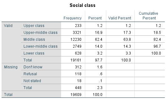
Out of all 19,161 respondents who provided a valid response when asked about their social class, what would be the probability of randomly selecting a middle-class person?
Going by the formula we’ve used so far, we have:
![\[p(\textrm{middle class})=\frac{\textrm{middle class N}}{\textrm{total N}}=\frac{12230}{19161}=0.638\]](https://pressbooks.bccampus.ca/simplestats/wp-content/ql-cache/quicklatex.com-8db4c6a3378f491cc7491c8347a44c4c_l3.png "Rendered by QuickLaTeX.com")
Or, the probability of randomly selecting a middle-class respondent from this group of people is 63.8 percent[1], exactly as the Valid Percent column tells us.
And what would be the probability of randomly selecting either an upper-class or an upper-middle-class person?


Or, the probability of randomly selecting an upper-class or an upper-middle-class respondent is 18.5 percent, as we can well see in the Cumulative Percent column.
Finally, what would be the probability of randomly selecting (with replacement) first a respondent who reported being lower class and then a respondent who reported being upper class?


Or, the probability of first selecting a person who reported being lower class and then a person who reported being upper class is a minuscule 0.004 percent. (A quick-and-dirty multiplication of the valid percentages of two groups, 1.2 percent and 3.3 percent, will give you the same result.)
See, it works! Now try it on your own.
Do It! 5.7 Marital Status (GSS 2016)
Look at Table 5.2 and answer the questions listed below.
Table 5.2 Respondent’s Marital Status (GSS 2016)
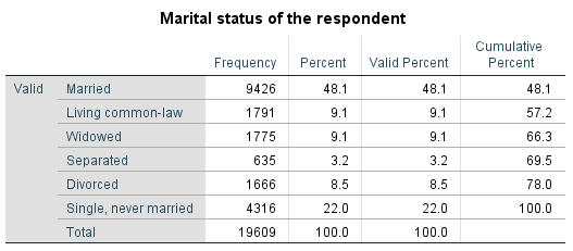
- What is the probability of randomly selecting a person (out of the 19,609 people) who is living common-law?
- What is the probability of randomly selecting a person (out of the 19,609 people) who is either separated or divorced?
- What is the probability of first randomly selecting a person (out of the 19,609 people, with replacement) who is married and then one who is single?
(Answer: 0.091; 0.117; 0.106)
In passing, we can also extrapolate that since percentages and proportions are relative frequencies, and probabilities are proportions and percentages, probability is relative frequency too.
- In Chapter 6 will will see that this is also the probability of a randomly selected Canadian (out of all Canadians) to be middle class, and why that is. This of course applies to all the calculations below. ↵