Chapter 10 Testing Associations II: Correlation and Regression
10.2.2 Elements of the Linear Regression Model
The secret to minimizing the residuals — and to ensuring the regression line is indeed the best fitting (to the data) line — lies in the way the elements of the line are calculated. The regression/preditcion line is, after all, created through a and b, as I explained in Section 10.2:
![\[\hat{y}=a+bx=\]](https://pressbooks.bccampus.ca/simplestats/wp-content/ql-cache/quicklatex.com-b8f7541da408bc5f6fb28eb3ee301981_l3.png "Rendered by QuickLaTeX.com")
= predicted values
We can calculate a and b such that they minimize the residuals through the following formulas:
![\[b=\frac{\Sigma{(x-\overline{x})(y-\overline{y})}}{\Sigma{(x-\overline{x})^2}}=\frac{SP}{SS_x}=\]](https://pressbooks.bccampus.ca/simplestats/wp-content/ql-cache/quicklatex.com-b3516c26a1e5d1de1949bbf65ea4072b_l3.png "Rendered by QuickLaTeX.com")
= slope, or regression coefficient
![\[a=\overline{y}-b\overline{x}=\]](https://pressbooks.bccampus.ca/simplestats/wp-content/ql-cache/quicklatex.com-ad420ab778d5cad52cd84be15928a9b1_l3.png "Rendered by QuickLaTeX.com")
= Y-intercept, or constant
where SP is, again, the sum of products, SSx is the sum of squares for x, and  and
and  are the variable means of x and y, respectively.
As with the correlation coefficient r, once again, everything revolves around variances (and means)[1].
An example will serve best to illustrate all this.
Example 10.3 Assignment Requirements and Marks
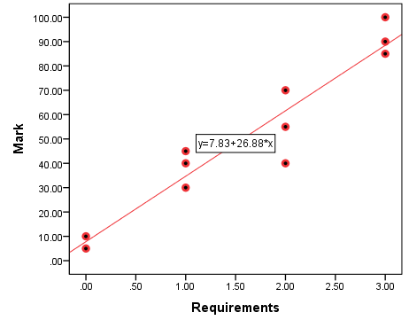
Here I continue with the fictitious data on which Figure 10.2 is based. In a “sample” of N=11, I have data about the “respondents”‘ completed assignment requirements (x) and their assignment marks (y). In Table 10.3, I calculate the necessary means, sums of squares, and sum of products.
Table 10.3 Assignment Requirements and Marks: Calculating a and b
 |
 |
 |
 |
 |
 |
 |
| 0 | 10 | -1.64 | 2.68 | -41.82 | 1748.76 | 68.43 |
| 1 | 40 | -0.64 | 0.40 | -11.82 | 139.67 | 7.52 |
| 2 | 70 | 0.36 | 0.13 | 18.18 | 330.58 | 6.61 |
| 3 | 100 | 1.36 | 1.86 | 48.18 | 2321.49 | 65.70 |
| 1 | 30 | -0.64 | 0.40 | -21.82 | 476.03 | 13.88 |
| 1 | 45 | -0.64 | 0.40 | -6.82 | 46.49 | 4.34 |
| 2 | 55 | 0.36 | 0.13 | 3.18 | 10.12 | 1.16 |
| 2 | 40 | 0.36 | 0.13 | -11.82 | 139.67 | -4.30 |
| 3 | 85 | 1.36 | 1.86 | 33.18 | 1101.03 | 45.25 |
| 3 | 90 | 1.36 | 1.86 | 38.18 | 1457.85 | 52.07 |
| 0 | 5 | -1.64 | 2.68 | -46.82 | 2191.94 | 76.61 |
 1.6 1.6 |
 51.8 51.8 |
SSx=12.55 | SSy=9963.64 | SPxy=337.27 |
Then, I substitute the relevant numbers into the formulas for a and b:
![\[b=\frac{SP}{SS_x}={337.27}{12.55}=26.88\]](https://pressbooks.bccampus.ca/simplestats/wp-content/ql-cache/quicklatex.com-7a746103c70938eea284a29c22a17e2b_l3.png "Rendered by QuickLaTeX.com")
![\[a=\overline{y}-b\overline{x}=51.8-26.88\times 1.6=51.8-43.99=7.83\]](https://pressbooks.bccampus.ca/simplestats/wp-content/ql-cache/quicklatex.com-6add20feed3b66e87aedc3552ab9c584_l3.png "Rendered by QuickLaTeX.com")
This makes our best-fitting/regression line this:
![\[\hat{y}=a+bx=7.83+26.88x\]](https://pressbooks.bccampus.ca/simplestats/wp-content/ql-cache/quicklatex.com-184103952e3bbcdeeaf583d830b03b8b_l3.png "Rendered by QuickLaTeX.com")
… which is exactly what SPSS had already told us, if you care to go back to Figure 10.2 in the previous section and check.
You may or might not be impressed by this, but you certainly need to know how to interpret it. In this case the regression tells us that a student who doesn’t complete even one requirement of their assignment is expected to receive 7.83 points (that’s the constant, or Y-intercept); further, for every requirement completed, their mark would increase by 26.88 points (that’s the regression coefficient). That is, the effect of one completed requirement on the assignment mark is 26.88 points.
We can also calculate the actual predicted values (which form the regression line itself):
- for x=0,
 ;
; - for x=1,
 ;
; - for x=2,
 ;
; - for x=3,
 .
.
As you can see, these are different values than the ones we had in the deterministic version with which we started in Section 10.1 (i.e., 0 requirements = 10 points, 1 requirement = 40 points, 2 requirements = 70 points, 3 requirements = 100 points). The difference between the certainty of the deterministic version and the uncertainty of the current probabilistic version is the unexplained (by number of requirements) variance[2]. How much variance we have explained we will see in the next section. Before that, here is Figure 10.2 again so that you can pinpoint the predicted values for yourselves. (Hint: they’re on the line.)
Figure 10.2 Assignment Requirements and Mark (Redux)
Testing the regression coefficient for statistical significance. Of course, as with any statistics obtained through a sample, we have to be able to check whether the regression coefficient is generalizable to the population, i.e., whether it is statistically significant. In other words, we have to examine the evidence whether the identified effect of the independent variable on the dependent variable exists in the population or whether it is a result of random sampling.
The significance test for b is your familiar t-test, given by the following formula[3]:
![\[t=\frac{b}{s_b}\]](https://pressbooks.bccampus.ca/simplestats/wp-content/ql-cache/quicklatex.com-2794fc0558ea76fa1669030b254867f5_l3.png "Rendered by QuickLaTeX.com")
where sb is b‘s standard error.[4]:
The degrees of freedom for tb are N-2 in the bivariate case. We can see what we can do with the test in hypothesis testing, next,
- So much so that the correlation coefficient r and the regression coefficient b are related:
 where sy and sx are, of course, the standard deviations of y and x, respectively. ↵
 - That is, in the deterministic version, we could say that
 (reality = prediction), or rather, that there is no prediction at all -- we know what the true relationship between the variables is as the assignment mark depends entirely on the number of fulfilled requirements. In the actual/probabilistic version,
  (reality = prediction plus residual/error), where the residual is what is left unexplained, or simply the difference between reality and prediction. ↵
 - The population version is
 . Since we generally do not know
  , we substitute it with its estimate, the sample-based sb. This of course also means we move to the t-distribution. ↵
 - The standard error of b is calculated by this, admittedly scary-looking, formula:
This can be simplified to be more user-friendly but then I will need to introduce additional concepts (like the mean squared error and the standard error of the estimate) which are not necessary for you at this stage and are therefore beyond the scope of this book. You will be happy to know that the hand calculation of sb also falls in that category. ↵![\[s_b =\sqrt{\frac{\frac{\Sigma{(y-\hat{y})^2}}{(N-2)}}{\sqrt{\Sigma{(x-\overline{x})^2}} }}\]](https://pressbooks.bccampus.ca/simplestats/wp-content/ql-cache/quicklatex.com-4a5ed7136608f9cf4357210baea33161_l3.png "Rendered by QuickLaTeX.com")