Chapter 10 Testing Associations II: Correlation and Regression
10.2.3 Hypothesis Testing and Confidence Intervals for the Regression Coefficient
To test the regression coefficient b for significance we have the following hypotheses:
- H0: The independent variable x has no effect on the dependent variable y (i.e., the variables are not associated); β=0.
- Ha: The independent variable x has an effect on the dependent variable y (i.e., the variables are associated); β≠0[1].
After calculating tb with df=N-2 and finding its associated p-value, we then compare the p-value to the pre-selected significance level α. As usual, when p≤α, we reject the null hypothesis, and have enough evidence to deem the regression coefficient b statistically significant. If, on the contrary, p>α, we fail to reject the null hypothesis and therefore conclude that at present there is no evidence to suggest an effect of x on y.
Again, similarly to other statistics, we can calculate confidence intervals for b, so that we can report the size of the effect with a specific level of certainty. For example, the 95% confidence interval for the regression coefficient b is:
- 95% CI:

To illustrate, let’s revisit our example about the effect of parental education on their offspring education. (Don’t worry, with N=1, 686 I will not offer you a calculation by hand: SPSS is there for us.)
Example 10.4 Effect of Parental Years of Schooling on Respondent’s Years of Schooling (GSS 2018)
We already examined the association between parental and offspring education through the correlation coefficient r and found it to be moderately weak at 0.413, and statistically significant at α=0.01. Can we do better, however, and estimate the effect of each additional year of parental schooling on the schooling of the respondents?
Again, we use data from the U.S. GSS 2018 (NORC, 2019). Our sample is N=1,686, and our hypotheses are:
- H0: Father’s education has no effect on respondent’s education; β=0.
- Ha: Father’s education has an effect on respondent’s education; β≠0.
The regression model is:

Our predicted values are:

Figure 10.3 plots the association and Table 10.4 show the relevant SPSS output.
Figure 10.3 Linear Regression of Respondent’s Years of Schooling and Father’s Years of Schooling
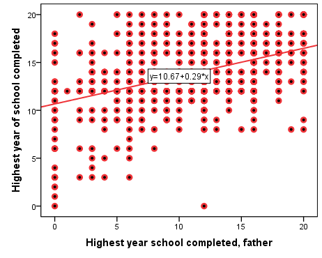
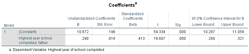
Table 10.4 Linear Regression of Respondent’s Years of Schooling and Father’s Years of Schooling
That is, SPSS has calculated the constant (or Y-intercept) a and the regression coefficient b in such a way as to minimize the residuals:
- a = 10.67
- b = 0.29
Then, the predicted values (i.e., the regression line on Figure 10.3 above) are:

We also know that the standard error of b is sb=0.016, so
![\[t=\frac{b}{s_b}=\frac{0.29}{0.016}=18.607\]](https://pressbooks.bccampus.ca/simplestats/wp-content/ql-cache/quicklatex.com-1d1f8cbd22fff3208117b67bb03cd621_l3.png "Rendered by QuickLaTeX.com")
Thus, with t=18.607, df=1,684, and p<α=0.001, we can reject the null hypothesis. Our current evidence supports our hypothesis that father’s education affects their offspring’s education, on average. The effect is 0.29 years (or about 3.5 months) for every additional year of father’s schooling, and it is statistically significant.
As well, we can interpret the confidence interval:
- 95% CI:
![\[b\pm1.96s_b =0.29\pm1.96(0.016)=0.29\pm0.031=(0.26; 0.32)\]](https://pressbooks.bccampus.ca/simplestats/wp-content/ql-cache/quicklatex.com-184ac451d0da4868a9242873f576722f_l3.png "Rendered by QuickLaTeX.com")
Or, father’s education’s effect on offspring’s education would be between 0.26 additional years and 0.32 additional years for every year of father’s schooling with 95% certainty; in other words, the effect would be 0.29 ± 0.031, 19 out of 20 times.
That’s a lot more information than simply stating that the variables are associated based on the correlation coefficient!
Now let’s make sure you understand how regression works and where the regression coefficients and line come from by interpreting regression output.
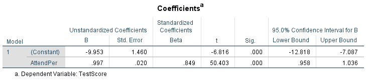
Do It! 10.2 Class Attendance and Final Test Scores (Simulated Data)
We are revisiting the simulated data on student class attendance (measured in percent of classes attended) and their final class scores. N=987. Start by stating your hypotheses, then, using the SPSS’s output presented in Figure 10.4 and Table 10.5 below, write a paragraph interpreting what you have found, discussing the evidence presented regarding your hypotheses and your decision about them, etc. Include as much information as possible, and do not forget to justify your use of linear regression in this case.
Figure 10.4 Class Attendance and Final Test Scores
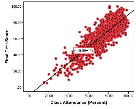
Table 10.5 Class Attendance and Final Test Scores
Finally, these are the steps through which the regression output is obtained in SPSS.
SPSS Tip 10.1 Linear Regression
- From the Main Menu, select Analyze, then from the pull-down menu, select Regression and click on Linear;
- Select your dependent variable from the list of variables on the left and, using the appropriate arrow, move it to the Dependent open space on the right;
- Select your independent variable from the list of variables on the left and, using the appropriate arrow, move it to the Block 1 of 1 empty space on the right.
- You can click OK or, if you need a confidence interval for b, click on Statistics, and check off Confidence intervals in the new window (here you can also specify the confidence Level of the CI); click Continue;
- Once back in the original window, click OK.
- After the OK, SPSS will provide the output in the Output window. The relevant information we have discussed so far can be found in the last table called Coefficients.
SPSS provides several tables as the standard regression output. Beyond the Coefficients one, there are three other short tables: a Variables Entered/Removed (which lists the independent variable/s in the model and the dependent variable as a footnote), an ANOVA table (which presents analysis of variance information that, as mentioned before, is outside the scope of this book), and a Model Summary table. We qill take a brief look at that last table in the next section.
- Note that I am using causal language here with the assumption that the conditions for causality are met. Theirs is a separate investigation. In and of itself, finding a significant effect of x on y does not itself establish that changes in x cause changes in y. ↵
- If you actually divide 0.29 by 0.016, you wil end up with 18.125. The difference from 18.607 is due to rounding (as the standard error of b is rounded up to 0.016 from 0.01558...). ↵