9.4 Between Two Discrete Variables: the χ2, Part 2

Mariana Gatzeva

Chapter 9 Testing Associations I: Difference of Means, F-test, and χ2 Test

9.4 Between Two Discrete Variables: the χ2, Part 2

Calculating a two-way χ² is only marginally more complicated than the one-way case we examined in the previous section, as Example 9.5 demonstrates.

Example 9.5 Do You Like The Campus Cafeteria? (Bivariate χ²-Test)

While we already know that year of study and opinion on the campus cafeteria are not statistically associated from the t-test in Example 9.3, I will further use the imaginary data in the original contingency table from Example 7.3 to demonstrate a two-way χ²-test. This was the table we had is Section 7.7.2.

Table 9.2 (A) Do You Like The Campus Cafeteria? (Revisited)

	First Year Students	Second Year Students	Total
YES	7	5	12
NO	8	15	23
Total	15	20	35

Our hypotheses are:

H₀: Liking the cafeteria or not is not associated with one’s year of study; first- and second-year students are equally likely to lie the cafeteria, or π₁=π₂.
H_a: Liking the cafeteria is associated with one’s year of study; first-year students and second-year students differ in their liking of the cafeteria, or π₁≠π_2.

To compute the χ², we need the expected count for each cell. Unlike the one-way χ² case, however, determining the expected count in a contingency table is a bit more complicated than dividing the N on the number of groups and expecting the same (expected) number in each cell. Instead, we multiply the respective group/category sizes (i.e., the row total and the column total at the margins) and divide the product by N (the full total)^[1]:

$f_e=\frac{N_j\times N_k}{N}$

where j is the size of the respective group and k is the size of the respective category^[2].

Thus we have the following:

First-years who said Yes: $f_e=\frac{N_j\times N_k}{N}=\frac{15\times 12}{35}=5.14$
Second-years who said Yes: $f_e=\frac{N_j\times N_k}{N}=\frac{20\times 12}{35}=6.86$
First-years who said No: $f_e=\frac{N_j\times N_k}{N}=\frac{15\times 23}{35}=9.86$
Second-years who said No: $f_e=\frac{N_j\times N_k}{N}=\frac{20\times 23}{35}=13.14$

Table 9.2 (B) adds the expected count in brackets next to the observed count.

Table 9.2 (B) Do You Like The Campus Cafeteria? (Observed and Expected Frequencies)

	First Year Students	Second Year Students	Total
YES	7 (5.14)	5 (6.86)	12
NO	8 (9.86)	15 (13.14)	23
Total	15	20	35

Now we only need calculate the four elements of the χ2 and add them altogether at the end.

First-years who said Yes: $\frac{(f_o-f_e)^2}{f_e}=\frac{(7-5.14)^2}{5.14}=0.67$
Second-years who said Yes: $\frac{(f_o-f_e)^2}{f_e}=\frac{(5-6.86)^2}{6.86}=0.5$
First-years who said No: $\frac{(f_o-f_e)^2}{f_e}=\frac{(8-9.86)^2}{9.86}=0.35$
Second-years who said No: $\frac{(f_o-f_e)^2}{f_e}=\frac{(15-13.14)^2}{13.14}=0.26$

Finally,

$\chi^2=\Sigma\frac{(f_o -f_e)^2}{f_e}=0.67+0.5+0.35+0.26=1.78$

The degrees of freedom are, again, df=(rows-1)(columns-1), so here df=(2-1)(2-1)=1(1)=1.

That is, with χ²=1.78, df=1, and p=1.18 (i.e., p>0.05), we do not have enough evidence to reject the null hypothesis. At this time, we cannot claim there is an association between year of study and opinion on the cafeteria, i.e., the 0.217 difference in proportions we observe in the sample (7/15 versus 5/20, or 0.467 versus 0.25) is not statistically significant.

Of course, we already knew this from the t-test in Example 9.3^[3], so no surprises here.

The imaginary example above serves well as a work-through for calculating χ², but we can do better — an example using real, random-sample data and a large N is in order.

If you recall, in Section 7.7.2 we also explored gender differences in the ability to speak an Aboriginal language using APS 2012 (Statistics Canada, 2019) data. Armed with knowledge about the χ², now we can finish that investigation.

Example 9.6 Testing Gender Differences in the Speaking Aboriginal Language Ability among Indigenous Canadians , APS 2012

Our exploration in Section 7.2.2 left us with the following table.

Table 9.3 Speaking Aboriginal Language Ability by Gender, APS 2012 (Revisited)

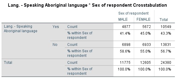
Our hypotheses are:

H₀: Gender and the ability to speak an Aboriginal language are not associated; women and men are equally likely to speak an Aboriginal language, or π_f=π_m.
H_a: Gender and the ability to speak an Aboriginal language are associated; women and men are not equally likely to speak an Aboriginal language, or π_f≠π_m.

SPSS calculates χ²as 31.78. With χ²=31.78, df=1, and p<0.001, we have enough evidence to reject the null hypothesis and conclude that Indigenous women and men tend to differ in their ability to speak an Aboriginal language. The 3.6 percentage points difference (i.e., 45 percent minus 41.4 percent) in favour of women being more likely to speak an Aboriginal language is statistically significant and therefore generalizable to the larger Indigenous population.

I “cheated” out of presenting the actual calculations in the example above to give you the opportunity to do it on your own. Use it as an exercise in practicing your understating of the χ² and t statistical significance tests.

Do It! 9.3 Testing Gender Differences in the Speaking Aboriginal Language Ability among Indigenous Canadians, APS 2012

Using the information presented in Table 9.3 above, 1) calculate the expected frequencies for each cell and compute the χ²; and 2) do a t-test on the difference of proportions and create a 95% confidence interval for the difference, to observe the correspondence between the different tests.

Finally, lest I leave you with the impression that there is no difference between using a t-test and a χ²-test, let’s consider a case where both variables have more than two categories, next.

We do that to account for the different group/category sizes. ↵
Recall that to differentiate between the groups/categories of the two variables, we refer to one variable having groups and the other having categories: so that we can say we compare the groups of one variable on the categories of the other. ↵
You may find it curious to know that the correspondence of results between the t and the χ² goes even further: in the binary variables' case, squaring the t-value will give you exactly χ²: t²=χ². In our examples, t=1.34, and 1.34²=1.79 which, if it was not for rounding, would be the same as χ². Even their respective degrees of freedom are the same, 1.8. This of course is not the case when at least one of the discrete variables has more than two categories. ↵

9.4 Between Two Discrete Variables: the χ2, Part 2

License

Share This Book