5.2.4 The Real Normal Distribution Is a Probability One

Now back to the normal distribution, as promised.

Recall, if you will, the distinction between discrete and continuous variables^[1]. Flipping coins and throwing dice and selecting respondents from a small number of categories are all discrete outcomes, so their probability distributions are also discrete.

On the other hand, continuous variables (i.e., mostly interval/ratio variables) have continuous probability distributions. The normal distribution — whose features we discussed at length — is one type of a continuous probability distribution.

As well, recall that probabilities are expectations. Thus, while some continuous random variables might have an approximately normal observed distribution, their probability distribution (i.e., expected in theory) is perfectly normal — because it’s theoretical.

I said it before and it bears repeating: just like a few coin flips can produce an unequal number of heads and tails despite the fact that the probabilities of getting heads or tails are both equal to 0.5 in theory, a variable can have an approximately normal frequency distribution while its probability distribution is theoretically normal. In short, we can expect some continuous variables to be normally distributed. For example, we can expect most people to be of average height or thereabouts, and to have few people who are much shorter or much taller, and the shortest and the tallest to be so rare as to be exceptional. 

This, however, is actually not why the normal distribution is so important in statistics. What do we care about “some variables” and whether their distribution is normal or only approximately so? (Well, we do use that information, of course, but that’s not the point here.) The reason the normal distribution is so valuable is because one specific very special distribution is normal — the sampling distribution, as we will see in Chapter 6. (The sampling distribution lies at the basis of statistical inference.) But let’s not get ahead of ourselves.

After all this, you can see the normal distribution as a normally distributed probability. (Or, instead of a frequency distribution, it is a relative frequency distribution). Thus, the area under the normal curve is equal to 1 (or 100 percent, the whole probability), and it can be sectioned off, as it were, to indicate various outcomes’ probabilities. See the following set of Figures 5.6.

Figure 5.6 (A) Probability of 1 (100%)

Figure 5.6 (B) The Mean Gives Us Two Identical (Symmetric) Parts of 50% Probability Each

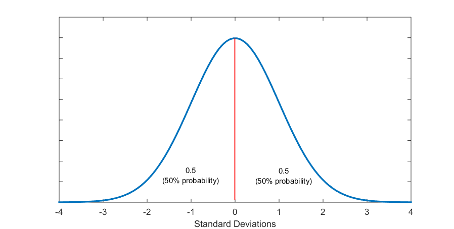
Figure 5.6 (C) 1 Standard Deviation from the Mean Sections Off  68% Probability

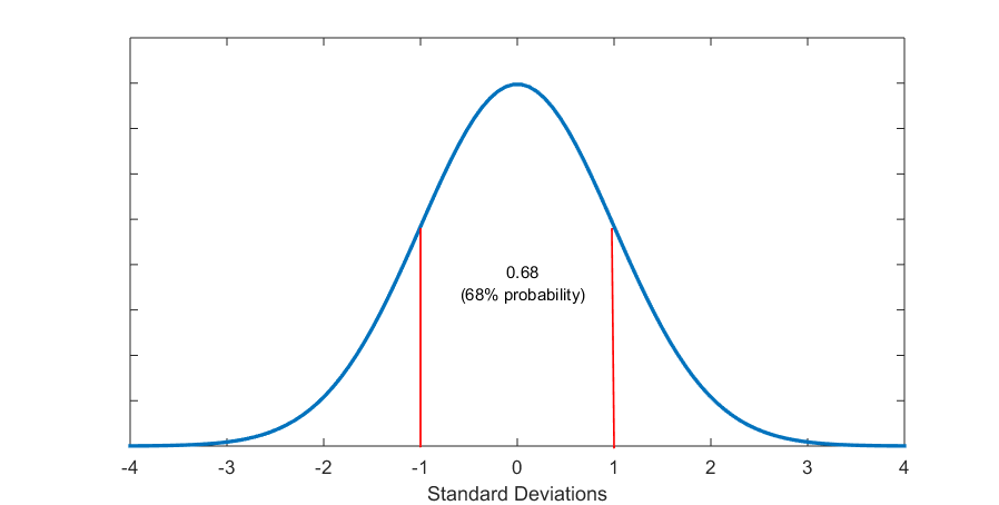
Figure 5.6 (D) About 2 Standard Deviations from the Mean Section Off 95% Probability

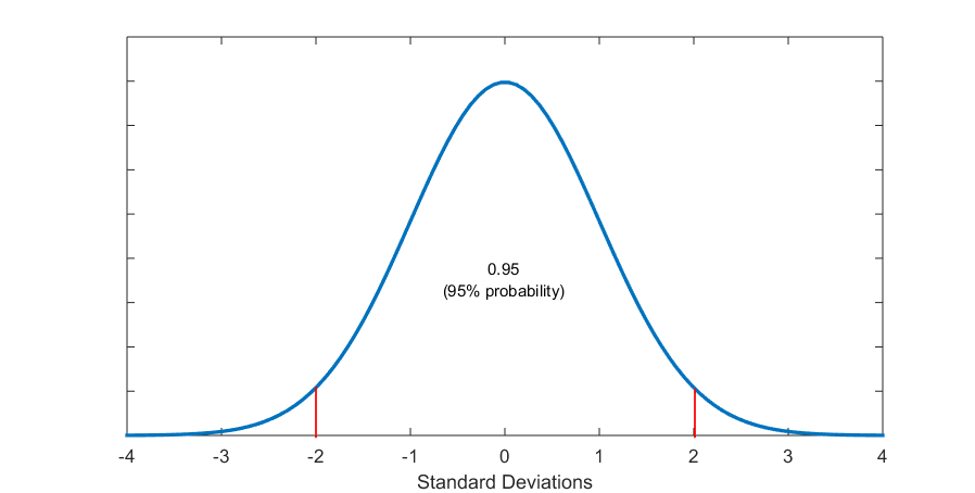
Figure 5.6 (E) About 3 Standard Deviations from the Mean Section Off 99% Probability

Thus, apart from what percentage of cases falls where, now we can discuss what the probability that a case will fall in a particular place is. Both refer to the same thing essentially but the latter indicates the theoretical expectation and allows us to be more precise (as empirically cases are only approximately normally distributed). Or, you can think of it like this: given the properties of the normal probability distribution, we can expect that much percentage of the data to be within that many standard deviations from the mean.

You’ll see how the normal curve allows us to calculate probabilities through z-values in the next and (to your eternal relief) final section on the topic.