Chapter 3 Measures of Central Tendency
3.3 The Median With Frequency Tables and Other Considerations
A similar — though far more widespread confusion – may happen when working with frequency tables. Frequency tables, as you know from Section 2.3.3 (https://pressbooks.bccampus.ca/simplestats/chapter/2-3-3-summing-up-adding-cumulative-percentages/), list a variable’s categories/values in the first column and their frequencies in the second column. Take a look at the incomplete frequency table of the fictitious number of siblings variable used from before.
Example 3.3 (B) Number of Siblings, Aggregated
Table 3.3 Frequency Table for Number of Siblings
| Value | Frequency |
| 0 | 1 |
| 1 | 2 |
| 2 | 2 |
| 3 | 1 |
| 4 | 1 |
| Total | 7 |
Can you as easily see that one of your (imaginary) friends has zero siblings, two of your (imaginary) friends have one sibling each, another two of them have two siblings each, etc.? While Table 3.3 presents the same information as Example 3.3 (A) in the previous section does, the way the data is organized is different, so again, make sure you differentiate the variable’s values (first column) from the values’ frequencies (second column).
A further consideration is finding the median itself. While we saw that the mode depended only on identifying the category/value with the highest frequency (and it was therefore just a matter of finding the largest number in the Frequency column of a frequency table), are you able to determine the median from the partial frequency table in Example 3.3 (B) above? I would venture that the answer would be “no” for most readers.
Of course, you can find a solution to our median-finding problem by “unpacking” the frequency column from Table 3.3 and reverting to raw (uncategorized) data again: one 0, two 1’s, two 2’s, one 3, and one 4 are 0, 1, 1, 2, 2, 3, 4. We already established (both visually and through using the position-of-the-median formula) that the middle case was Case #4, or “two siblings”. Would you like, however, to do that for the following Table 3.4?
Table 3.4 Household Size of the Respondent (GSS 2016)[1]
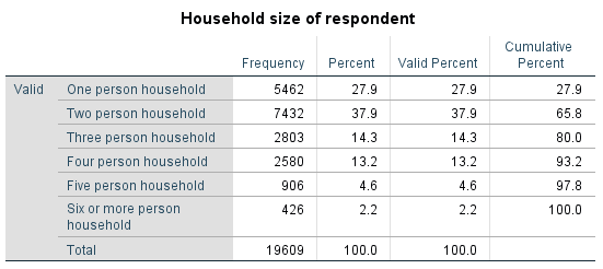
Most likely, you wouldn’t “unpack” the 19,609 cases into raw data, so we should seek some other — and more generalizable — method for finding the median through frequency tables, one that would apply to N of any size.
We could, of course, use the formula to at least establish the middle case’s numbered position, and then work our way through the table to identify the median.
![\[\frac{N+1}{2}=\frac{19,609+1}{2}=\frac{19,610}{2}=9,805\]](https://pressbooks.bccampus.ca/simplestats/wp-content/ql-cache/quicklatex.com-4a6927158f9a4389dc8507c17ac9922c_l3.png "Rendered by QuickLaTeX.com")
That is, Case #9,805’s household size will be the median household size for these almost 20 thousand respondents.
How do we find it? There are 5,462 respondents who reported living alone (“one person household”) so we know that Case #5,462 does not “reach” the median yet, thus we have to count further. We take the next 7,432 respondents who reported living in two person households, but we need to add them to the 5,462 people living alone in order to obtain the second group’s case number positions. After all, the case count for the 7,432 respondents does not start from 1 but from 5,463, and Case #5,463 will already be living in a two person household. So will Case #5,464, Case #5,465, etc. … all the way up to Case #12,894 (because 5,462+7,432=12,894), which will be the last respondent living in a two person household.
However, we now see that we have “counted” too far ahead — we have jumped not to Case #9,805 but all the way to Case #12,894! We do know though that all cases between Case #4,463 and Case #12,894 live in two person households: this is enough for us to establish that Case #9,805 lives in a two person household as well.
In short, the median household size of the 19,609 respondents is two-persons household. That is, half of the respondents live in two-person or smaller households and half of them live in two-person or larger households.
Hmm, I hear you say, this is still quite the roundabout way of getting to the median — can you do better?
Alright, let’s think of something else then. We tried adding the frequencies together until we reached the median… How about we try using percentages this time around — and more to the point, cumulative percentages, as they are already keeping a running total? We just need to know which percent corresponds to the middle case.
Recall, then, that the middle case splits the distribution of the cases in two equal halves. What percent is half of something? Of course, 50 percent. Thus it would make sense to simply look at the Cumulative Percent column and try to figure out where 50 percent would fall. The respondents living alone comprise 27.9 percent, so too low for the median, but the respondents living in one or two person households added together comprise already 65.8 percent of the total. Following the same logic as with the frequencies, the 50th percent falls within the one/two person household cumulative group. However, we know it’s not within the one person household group. That means the 50th percent can only fall within the respondents living in two person household, which, again confirms what we already knew: the median household size is made up of two persons.
To generalize, if you’d rather not use the formula for the median’s position and add the frequencies of a frequency table up in order to find the median, you can always simply look for within which category/value the 50th percent would fall. That category/value will be the median one.
Do It! 3.3 Median Workplace Size
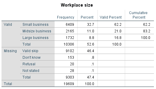
Let’s revisit Table 2.6 from Section 2.3.4 (https://pressbooks.bccampus.ca/simplestats/chapter/2-3-4-what-frequency-tables-look-like/). Can you identify the median of workplace size? And since you’re at it anyway, what about the mode?
Imagine you have to tell what you have found to some of your friends who have no knowledge of statistics. How are you going to explain to them your findings about the mode and the median of workplace size?
Table 2.6 Frequency Table for Workplace Size of the Respondent (GSS 2016)
Finally, now that you have learned what the median is and how you can find it, I will also casually mention that you can use SPSS for that. (Okay, okay. Don’t throw bricks, please: it really is important to work through the examples and exercises manually so that you understand what the SPSS output tells you and so that you are able to interpret that output properly.)
SPSS Tip 3.3 Finding the Median Of a Variable
- From the Main Menu, select Analyze, then Descriptive Statistics, then Frequencies;
- Select your variable of choice from the list on the left and use the arrow to move it to the right side of the window;
- Click on the Statistics button on the right;
- In this new window, check Median of the Central Tendency section on your right;
- Click Continue, then OK.
- The Output window will provide a small table listing the median of the selected variable.
Keep in mind that the Watch Out!! #6 warning from Section 3.1 about the mode applies equally to the median: for ordinal variables, SPSS will provide the median in numerical code. It is your job to “translate” the code into the actual category’s name. In the case of household size SPSS supplies “2” as the median, which stands for “two person household”. Thus we say that the median household is a two-person one; we do not report that the median household is “2”.
Watch Out!! #7… for Misinterpreting the Formula for the Median
An extremely common mistake regarding the median is to take the result of  to be equal to the median itself. This is patently not true. Again, what the formula provides is the place (or the numbered position) of the median once the cases have been put in their correct order:
![\[\frac{N+1}{2}=\]](https://pressbooks.bccampus.ca/simplestats/wp-content/ql-cache/quicklatex.com-e31ba6b300acc936c36f20105473091f_l3.png "Rendered by QuickLaTeX.com")
“numbered position of the median case in the ordered list of cases”
Thus, once your calculation for the place of the median is done, do not forget to do the final step: check the position you have calculated and see what the category/value of the median case is. You need to report only that value, not the position itself.
Stability of the median. A final noteworthy observation about the median is its stability as a measure of central tendency. Since the median is entirely about the central position in a variable’s distribution and all it takes into account is the order of the cases, not their substantive values, it’s impervious to the actual magnitude of the values. Thus it doesn’t matter if we have a set of values like 1, 5, 20, or one like 4, 5, 6, or another like 0, 5, 9 — the median is the same for all three, even if the values in the sets are different. Whether we have a small or a large value is immaterial, all that it matters is where the value goes into the order of the variable’s cases.
You will learn why this has important implications for the central tendency in the next section, all devoted to the mean.
- Note that this variable is technically an ordinal variable. Despite the numerical values and equal "distances" (of one person) between the first five categories, the last category "Six or more person household" prevents us from categorizing the variable as ratio. After all, we don't know exactly how many individuals live with any of the 426 people in that category: it could be six, or seven, or eight, etc. Thus it is not possible to say how many more persons live in the households of the respondents in the last category compared to any of the preceding categories: the "distance" is no longer one person. Any interval/ratio variable that has its last category truncated in this way (i.e., it has "... or more" in its label) becomes technically ordinal. Nevertheless, for heuristic purposes I will ignore the "...or more" part in this example which allows me to assume that everyone in that last category lives in a six-person household. This, in turn, allows me to pretend the variable is a ratio. However, the example works the same way regardless if the variable is truly ordinal or ratio. ↵