Chapter 9 Testing Associations I: Difference of Means, F-test, and χ2 Test
9.2 Between a Discrete and a Continuous Variable: The F-test
When the discrete variable of interest has more than two categories, we can no longer use the simple t-test presented in the previous section. While we can still use a boxplot chart for visualizing the association between the two variables — where instead of two boxplots, we will have as many boxplots as there are groups (categories of the discrete variable) — we no longer have only one difference to test.
Testing multiple means for statistical significance is done through a version of a test called an F-test. This F-test tests whether the means of several groups[1] are all equal (versus at least one of them not being the same as the rest) through an analysis of variance (aka ANOVA).
At this point you might feel like a treatment of the topic of the kind I offered about the t-test above would be a tad too much, and you will be correct: providing the full-on technical details and the formula of the F-test is beyond the scope of this book.
Briefly, the ANOVA F-test calculates a ratio of variances (between groups to within groups, in terms of sums of squares): the larger the ratio, the more evidence there is against the null hypothesis, and vice versa. The F-test statistic follows an F-distribution (not discussed here), which provides the F-value with its p-value, which is then compared to the α-level and interpreted in the usual way. Example 9.2 illustrates.
Example 9.2 Education Differences in Average Income, NHS 2011
Presumably, college is worth it. You delay your full entry into the labour force and instead invest in your education, with the hope that you will then be able to have a better — and better–paying job.
Let’s examine this questions then — do higher educational degrees translate into higher average income? — using about 3 percent random sample of the NHS 2011 data. The variable income is the same one I used in previous occasions (i.e., total income in NHS 2011). The groups to compare are the categories of a variable called (highest) degree. The variable degree is a recoded version of the NHS 2011‘s highest certificate, diploma or degree. I recoded the original variable’s thirteen categories in degree‘s six: 1) no high school, 2) high school, 3) certificate or diploma below Bachelor’s, 4) Bachelor’s, 5) Master’s[2], and 6) PhD.
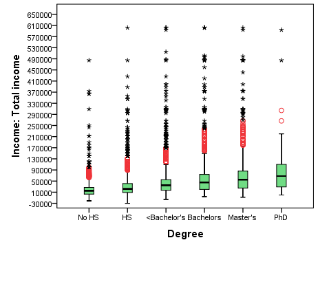
A brief descriptive investigation of the data reveals that the average income reported by the six education groups looks different: \$19,433 for respondents without a high school degree, \$30,455 for respondents with a high school degree, \$41,971 for respondents with more than a high school but less than a Bachelor’s degree, \$60,360 for respondents with a Bachelor’s degree, \$71,593 for respondents with a Master’s degree, and \$93,924 for respondents with a PhD. This potential positive association (more education, more income) is also reflected in the boxplots in Figure 9.1. While there are outliers with extremely high average income in all groups (the most extreme were even truncated at the top), the median and the outlier-less maximum income increase from left to right with the increase of highest degree.
Figure 9.1 Average Income by Highest Degree, NHS 2011
Are these differences statistically significant? In other words, are the differences observed in the sample a result of regular sampling variation, or reflective of differences in the population?
- H0: The average income of all six education groups is the same.
- Ha: The average income of some of the education groups is different from others.
SPSS reports a larger between-groups than within-groups variance; F=413.535 with p<0.001. With the probability of observing such differences between the groups in the sample — had there been no difference in the population (i.e., under the null hypothesis) — less than 1 in a thousand, we reject the null hypothesis and conclude that the differences in average income of groups with different highest degrees are statistically significant.
Before we turn to testing associations between two discrete variables, the SPSS Tip 9.1 below lists the steps of the t-test and ANOVA F-test procedures.
SPSS Tip 9.2 The F-test
- From the Main Menu, select Analyze, and from the pull-down menu, click on Compare Means and then One-Way ANOVA;
- Select your continuous variable from the list of variables on the left and, using the top arrow, move it to the Dependent List empty space on the right;
- Select your discrete variable from the list of variables on the left and, using the bottom arrow, move it to the Factor empty space on the right; click OK.
- The Output window will present a Oneway ANOVA table, listing a breakdown of variances (by sums of squares), and most importantly, the resulting F-statistics and p-value.
- Note that "several groups" includes the two-groups case as well: you could test the significance of a difference between the means of two groups with an F-test too (it will just provide less information). ↵
- This category includes certificates above Bachelor's, and medical, dentistry, and veterinary degrees. ↵