6.7 Confidence Intervals

In our discussion on statistical inference so far, I have used not one type of estimators but two, without bringing your attention to it. Probability theory and the Central Limit Theorem describing the sampling distribution of statistics provide us with two types of estimators, called point estimators and interval estimators.

A single sample statistic which estimates a population parameter — and which offers a “best guess” for that parameter — is a point estimator. We have worked with several point estimates by now: the sample mean is a point estimate of the population mean μ while the sample standard deviation s is a point estimate (which we can note as ) of the population standard deviation σ.

Similarly, I’ll add another useful point estimate, of the sample proportion. Imagine we are interested in studying unemployment. We take a random sample which reveals that, say, 10 percent of the sample respondents report being unemployed. Thus, we have the sample proportion p as 0.1 and we can use that proportion as a point estimate of the proportion of the population which is unemployed. We denote population proportions by the small-case Greek letter for p which is π^[1]. In other words, the sample proportion p serves as a point estimate of the population proportion π.

You’ll be happy to know that you are also already familiar with the other, interval, type of statistical estimators. As their name suggests, interval estimators, called confidence intervals, provide not just one number as a best guess but a whole set of plausible values for the population parameter.

If you recall Examples 6.3 and 6.4 from the previous section, you’ll recognize that we already calculated confidence intervals. In Example 6.4 on the average annual salary, we found a range of values within which the average annual salary of the city population was estimated to fall. Specifically, the average annual salary of the random sample was $50,000 and we were able to estimate with 95% certainty that the average annual salary of the city population would fall between $49,400 and $50,600. This range of values between $49,400 and $50,600 is in effect a confidence interval (a 95% confidence interval, to be precise). The actual numbers “bracketing” the interval are called error bounds; the interval itself is between, and including, the lower error bound and the upper error bound. 

Up until now, we calculated the confidence interval in a fast and easy way as I wanted to get the point of the logic underlying statistical inference across. At this time, however, we need to get more technical and precise about it.

First, let’s revisit how we did it in the previous section to refresh your memory; then I’ll show you the more correct way to do it. (Before you panic, know that what we did before was not incorrect; we just used rounded numbers to make calculations easier/faster.)

This is the information about the sample mean and standard deviation we had from Example 6.4 Average Annual Income (without the dollar signs for clarity of presentation):

Our starting point is the sample mean (which, according to the CLT approximates the population mean, with large N). In order to calculate a confidence interval around the sample mean , we first need to get the standard error , given by the CLT-based formula:

We don’t know the population standard deviation but we estimate it with its point estimator s, so we get:

Substituting s and N in the formula gives us the following:

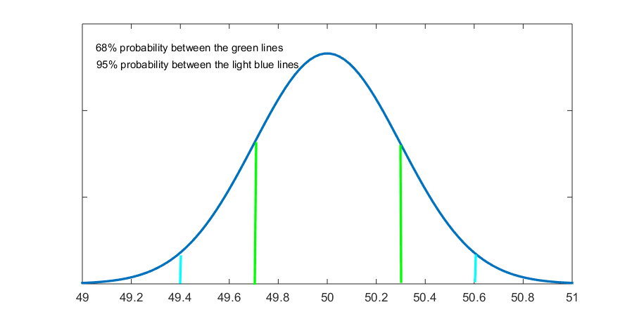
Now, by the CLT, we have everything we need for the sampling distribution: its mean (as estimated by the sample mean , its standard deviation (i.e., the standard error ), and its shape as a normal curve. From Section 5.2.4 (https://pressbooks.bccampus.ca/simplestats/chapter/5-2-4-the-real-normal-distribution/), we know the probabilities under the normal curve, and that 68 percent of cases^[2] fall within 1 standard deviation from the mean while 95 percent of cases fall within about 2 standard deviations from the mean.

The resulting graph was presented in Fig. 6.2 in the previous section. Here it is again, this time with the 68 percent demarcations included.

Figure 6.3 Average Annual Income (in thousands of dollars), Revisited 

However, to calculate a confidence interval we don’t need to draw the sampling distribution every time; we just need to keep in mind what it represents in terms of probabilities.

From our discussion of Example 6.4 in the previous section and now, we can easily deduce the basic formula for calculating a confidence interval:

• for a 68% confidence interval around the mean, we would have
  • 
• for a 95% confidence interval around the mean, we would have
  • 

We could even add the 99% confidence interval, encompassing values within about 3 standard deviations away from the mean:

• for a 99% confidence interval, we would have
  • 

Using the data from Example 6.4 for illustration, we then have the following confidence intervals (CI):

• 68% CI: 
• 95% CI: 
• 99% CI: 

Fig. 6.4 illustrates these confidence intervals.

Figure 6.4 Confidence Intervals for Average Annual Income

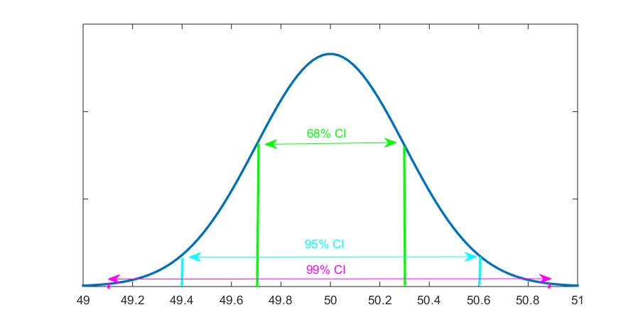
That is, we find that the average annual income for the city population is between $49,700 and $50,300 with 68% certainty; it is between $49,400 and $50,600 with 95% certainty; and it’s between $49,100 and $50,900 with 99% certainty. Alternatively, we could report that the average annual income of the city population is $50,000 ±$300 with 68% confidence; $50,000 ±$600 with 95% confidence; and $50,000 ±$900 with 99% confidence.

The (i.e., the plus and minus the estimated standard error) represents the margin of error for the specific confidence interval.

Now that you understand the principle of calculating confidence intervals, let’s start doing it with greater precision, as we normally would in real-life research.

Even if I used “1, 2, 3 standard deviations/errors away from the mean” in the calculations so far, this is a quick-and-easy rounding only approximating the real formula for confidence interval. From Section 5.2.5 (https://pressbooks.bccampus.ca/simplestats/chapter/5-2-5-the-real-use-of-z-values/), we know that the probabilities under the normal curve are associated with specific z-values.

If you check the z-values (standard normal distribution) table^[3], you’ll actually see that the precise z-values associated with 95% probability^[4] and 99% probability^[5] are 1.96 (almost but not quite 2) and 2.58 (almost but not quite 3), respectively.

Now you know that even if the z-value associated with 68% probability^[6] is indeed 1, the other two confidence intervals we have used so far need to be recalculated properly:

• 68% CI: 
• 95% CI: 
• 99% CI: 

To interpret, we find that we can be 95% certain that the average annual income of the population is between $49,412 and $50,588. As well, we find that we can be 99% certain that the average annual income is between $49,226 and $50,774.

Furthermore, although going by “1, 2, 3 standard deviations/errors” makes intuitive sense, in reality would you be happy to learn anything “with 68% certainty”? Sixty-eight percent certainty is hardly certain at all! (As such, it is pretty much never used outside of teaching.)

On the other hand, while the 95% and 99% confidence intervals are the most widely used and useful ones, there is no need to restrain yourself, should you choose to calculate any confidence interval you wish.

The general formula for a confidence interval is thus:

• Any % CI: 

To calculate this, you need to choose the level of certainty you want; once you have the probability, (divide it by two and) check its corresponding z-value, then multiply it by the standard error to get the margins of error with the desired probability level of certainty.

For example, I might want the 90% CI (not as popular as the other two but still a relevant confidence interval that has its uses).

I check for the z-value associated with 90% probability^[7] in a z-distribution table and I find that it’s 1.65. Then, for the example used above, I would get:

• 90% CI: 

Or, I can be 90% certain that the average annual income of the population of that city is between $49,505 and $50,495.

By analogy, you can thus produce any confidence interval with any level of certainty you want.

A bit more on confidence intervals in the next section.