Chapter 6 Sampling, the Basis of Inference
6.8 The t-Distribution
If, having reached this chapter’s final section, after all we had been through, random sampling, sampling distribution, CLT, parameters, estimates, statistics, confidence intervals, you are now groaning in dismay — why is there even more to this topic??[1] — take heart, this is a short explanation I kept for last, through a brief introduction of new concept.
If you recall, when we needed to calculate the standard error of the mean (or proportion) in the previous few sections, I simply replaced the unknown population standard deviation σ with the known sample standard deviation s in the formula. This is what I did:


Substituting in s for σ we had:


Similarly, for the proportion we had

and substituting the known sample proportion p for the unknown population proportion π in calculating the proportion’s variability, we ended up with:

But why can we do that?
The more observant of you might have noticed that I swept the explanation for this change under the carpet and simply moved on — but why should the variability of the population be the same as the sample?
In truth, they are not — or rather, they might be; there’s just no way to know. That is, by using the sample statistics to estimate the variability of the population, we introduce more uncertainty in the calculation. When we do that, we actually move away from using the normal distribution and its associated z-values. What we end up using is something similar, called the t-distribution[2]: an entire set of bell-shaped curves, accounting for each and every sample size N. Figure 6.5 illustrates.
Figure 6.5 The Normal vs. the t-Distribution
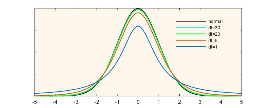
The t-distribution provides a separate bell-shaped curve for each possible sample size, thus helping us “ground”, as it were, the estimation in the reality of an actual sample of a specific size.
The accommodation of the sample size is done through the concept of degrees of freedom (commonly abbreviated to df). The degrees of freedom represent the number of values in a statistical calculation that are free to vary. In the case of the t-distribution, the degrees of freedom are N-1 as one degree of freedom is reserved for estimating the mean, and N-1 degrees remain for estimating the variability. Unlike with z-values, where each z-value represents a specific probability under the normal curve, the probabilities associates by t-values are calculated based on its degrees of freedom.
Still, none of this explains why I was able to shamelessly switch from using the z-distribution to the t-distribution, without any change to the standard error and confidence interval calculations in the examples in the previous sections. If z-values and t-values (and their associated probabilities) are different, shouldn’t the calculations differ too?
Before I reassure you that all is well (and it is), let’s revisit what z-values actually represent. From Chapter 5 you know that the z-value is the distance between a case and the mean, expressed in terms standard deviations (i.e., standardized):
![\[z=\frac{x_i-\overline{x}}{s}\]](https://pressbooks.bccampus.ca/simplestats/wp-content/ql-cache/quicklatex.com-7bb9bffb532f78ef46d182a25a8141d6_l3.png "Rendered by QuickLaTeX.com")
The reason we were able to use z=1, z=1.96, and z=2.58 in the calculations of the 68%, 95%, and 99% confidence intervals, respectively, was because the sampling distribution is a normal distribution (per the Central Limit Theorem). That is, the z-value in this case is the distance between the sample mean (the “case” in the sampling distribution) and the population mean (“the mean of means”, the mean of the sampling distribution), expressed in standard errors (the “standard deviation” of the sampling distribution):
![\[z=\frac{\overline{x}-\mu}{\sigma_\overline{x}}\]](https://pressbooks.bccampus.ca/simplestats/wp-content/ql-cache/quicklatex.com-a301ef5bee38821a2d001f3210733249_l3.png "Rendered by QuickLaTeX.com")
Now what about t? By substituting the sample standard deviation for the population standard deviation, we end up with the estimated standard error. In turn, substituting the estimated standard error for the standard error in the formula for the z-value above, we get the t-value, the distance between the sample mean and the population mean, expressed in estimated standard errors:
![\[t=\frac{\overline{x}-\mu}{s_\overline{x}}\]](https://pressbooks.bccampus.ca/simplestats/wp-content/ql-cache/quicklatex.com-25e3f98e722f4d2c1a4172301778750d_l3.png "Rendered by QuickLaTeX.com")
Compare the two formulas for the z-value and the t-value above. As similar as they look, the t-value is more “uncertain” than the z-value, and comes with the aforementioned specification of degrees of freedom. Given specific degrees of freedom, the shape of the t-distribution curve changes, and thus the probabilities associated with each t-value change too.
Finally, for the drum roll: The reason I was able to work with t-values instead of z-values in the calculations of confidence intervals in the previous section without acknowledging it is due to the sample sizes I chose for my examples. See, the biggest difference between the z and the t happens with small N (especially N<30). The larger the N, the closer and closer the t-distribution approaches the z-distribution.
You can see this in Figure 6.5 above: as the degrees of freedom increase, the shape of the distribution becomes more and more normal, so much so that the t-distribution at df=30 is already rendered invisible in the figure, its light blue colour overridden by the normal distribution’s black. And from N=100 on, the t converges so fast to z, the t-distribution curve becomes our old, familiar, beloved normal curve! (Okay, maybe “beloved” applies just to me.)
Given that in the confidence interval examples in the few preceding sections I used only large N‘s (=900 and above), the probabilities associated with the t-value at N-1 degrees of freedom (=899 and above) were the same as those associated with the z-values: 68% for t=z=1, 95% for t=z=1.96, 99% for t=z=2.58. (Hence I left them out of the discussion at that time to properly explain here.)
Hmm, much ado about nothing, I can imagine you saying at this point. If the t-distribution and the z-distribution are no different at larger N, why even bother with the t (beyond any small-N uses)? And as unsatisfying the answer “I’ll explain later” is, I’m afraid I have no choice but to resort to it, again. Briefly, it has to do with something called a t–test for significance which we will be using soon enough for hypothesis testing in Chapter 7, next.
For now, what you should take away from this section is that the t-distribution exists, and it is what we actually use for estimation (and not z!), given a specific sample size. As well, remember that for N=100 and above, t converges to z so you can readily apply any probabilities you associate with z to t with N-1 df. (Regarding the latter, do not forget to always specify the degrees of freedom for whatever t you might have. A t-value always comes with df attached as it’s meaningless/undefined without them.)
- As a general principle, in introductory texts such as this there is always more. Much, much more; it's not a matter if but of how much something is left out. ↵
- Also called the Student's t-distribution, after the pseudonym of William Gosset who introduced it to statistics (along with many other concepts). Due to contractual obligations, William Gosset used to publish under the name of "Student" (Pagels, 2018). Here you can find more about his curious case: https://medium.com/value-stream-design/the-curious-tale-of-william-sealy-gosset-b3178a9f6ac8. ↵
- where
 . ↵
. ↵ - Where

 . ↵
. ↵