10.2.4 R-squared

In the previous section we established that the correlation coefficient r and the regression coefficient b are related:

And how could they not be: if a slope exists, a correlation exists. As such, the standard regression output provided by SPSS includes a Model Summary table that lists the Pearson’s r. Table 10.6 below is the Model Summary table of the simulated-data class attendance/final class scores regression.

Table 10.6 R and R² for Class Attendance and Final Class Scores

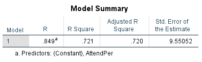
Pearson’s r (listed as R) in this table is, of course, exactly the same as what the SPSS Correlate procedure provides. Squaring that number, however, provides us with a new and useful piece of information, sometimes called the coefficient of determination, but more often simply referred to as R².

R² provides a measure of the proportion of the variability in the dependent variable explained by the independent variable[footnote]Or, independent variables, in the case of multivariate regression.[/footnote] in the model.

Recall that regression’s logic is based on minimizing residuals/errors and about explaining the variation of the dependent variable through information about the independent variable. In a deterministic case, the dependent variable will depend entirely on the independent one, and then we would have a correlation of 1 and R²=1. However, with uncertainty and estimation, this is not the case — some variability of the dependent variable remains unexplained by the regression model (i.e., the independent variable).

Thus, one way to look at R² is as an indication of goodness of fit: how close the observations are fitted around the regression line (i.e., how little variability is left unexplained). The larger R² then, the better — as a large R² would mean the model (the independent variable/s) explains a large proportion of the variability in the dependent variable.

As you can see in Table 10.6 above, the R² of the class attendance/final test scores is:

Or, class attendance explains 72.1 percent of the variability in final test scores, which is a lot, and quite good regression fit^[1].

Compare this to the Model Summary table of respondent’s and father’s years of schooling in Table 10.7 below.

Table 10.7 R and R² for Respondent’s and Father’s Years of Schooling

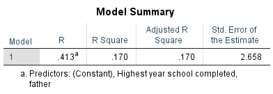
Unlike the very strong correlation of r=0.849, the moderately weak correlation coefficient r=0.413 is already an indication of not that great a fit. Thus, the R² of offspring and parental education is:

That is, fathers’ years of schooling explain only 17 percent of the variation of respondents’ years of schooling. The biggest ‘chunk’ of the variation in schooling is left unexplained, i.e., there are other factors influencing how much education one is expected to have, on average. Regardless, we should not dismiss parental education outright — it still has a statistically significant effect on offspring education (albeit not very strong).

. . . Or does it? Recall our discussion on causality. The fact that two variables are statistically associated does not necessarily mean that one causes the other to change (or, that it explains the other’s variability). Working with only two variables prevents us from accounting for alternative explanations — i.e., of taking into account other factors, other variables, other effects. Luckily, regression has our backs. I leave you with how that happens in the next — and final! — section of this textbook.