Chapter 6 Sampling, the Basis of Inference
6.6 The Central Limit Theorem
Despite it’s scary-sounding name, the Central Limit Theorem (CLT) simply describes the sampling distribution — and simultaneously explains why, and how, we can use sample statistics (like the mean of a variable,  , obtained through sample data) to estimate population parameters (like the true population mean of that variable, μ).
Recall what we use to describe a variable’s frequency distribution: 1) a graph to visually display the distribution’s shape; 2) measures of central tendency; and 3) measures of dispersion. In the previous section I also asked you to imagine the (entirely theoretical, i.e., probability) distribution of the mean (again, in theory, over infinitely repeated samples). What the CLT does then is provide information about all three of these elements (shape, central tendency, dispersion) but about the distribution of mean. In short, the CLT describes the sampling distribution of the mean.
The sample size plays an important role: the CLT applies to “large N”, and is stated for “as the sample size grows”, bringing us back to the point that the larger the N, the better for inference it is.
Specifically, the CLT states that with random sampling, as N increases (i.e., for large N), the shape, central tendency, and the dispersion (of the sampling distribution) of the mean, , will be the following:
- The distribution of will approach normal distribution in shape. (That is, the sampling distribution is a bell-shaped curve.)
- The mean of the sampling distribution[1] (denoted as
 ) will become the population mean,
  . (That is,
  .)
.) - The standard deviation of the sampling distribution (denoted as
 ) is called the standard error, and is related to the population standard deviation, σ, by the formula
  .
.
This may seem like a lot to take in (what with all the jargon, notation, and all) but it really is simply a description of a distribution. The next paragraph clarifies each of the CLT’s points in turn.
As brief as it is, the CLT is conveniently packed with all sorts of useful information: The sampling distribution is normal in shape — so we can apply all we know about the normal distribution to it (for example, that it’s bisected by its mean). Hence, the sampling distribution is centered on the population mean. Finally, according to the formula for the sampling distribution’s standard deviation (a.k.a the standard error), as the sample size N grows, the standard error becomes smaller[2] — so the distribution will be less variable/spread out, and thus the estimates will be closer to the parameters[3].
To summarize, the sampling distribution provides us with a bridge between sample statistics (i.e., estimators) and population parameters (i.e., the estimated). The CLT provides a description of the sampling distribution: by giving us information about an estimator (in hypothetical repeated sampling), it decreases the uncertainty of the estimation since now we can calculate how close the statistic is to the parameter.
I say estimator and statistic, not mean, because CLT (or a version thereof) applies to all statistical estimators, as they all have a normal distribution with increasing sample size. The latter is noteworthy because it’s true regardless of the shape of the original variable’s distribution (in the population): a variable might not be normally distributed but its mean (and other statistics) always is.[4]
If you are wondering about the connection between random sampling and the normal distribution, the following video might help:
The video above uses a Galton board to demonstrate the connection between randomness and normal curves by showing that balls falling randomly end up distributed approximately into a bell-shaped curve — with the majority in the centre, fewer to the sides, and fewer yet in the “tails”. You can think of a sample mean as one of these balls (all other balls are the means of other samples of the same size). Thus, what we see is that the majority of means would fall in the centre, fewer to the sides, and fewer still in the tail ends. However, since we do not have many means at all but only one, produced by one sample, we are dealing with a probability distribution. In turn, this tells us that the highest probability is the mean to fall in the centre region, with smaller probability to be to the sides but still close to the centre, and a further decreasing probability the farther it gets from the centre, just like with any probability normal curve[5].
If you still find all this hopelessly abstract (as I’m sure most do), you can see exactly how we use the CLT for inference in the example below. (Unfortunately, your relief to be back to examples will be premature at this point: we have more necessary theory to cover ahead. On the bright side, we are more than half-way in the chapter so cheer up, the end is near.)
As a heads-up, here’s the rationale of what we’ll do: In order to explain inference about populations based on samples, we’ll reverse-engineer it. That is, we’ll start with “knowledge” about the population and, based on the CLT, we’ll “infer” the sample statistic. At the end we’ll see that following the same logic (but in reverse) we can easily do the opposite — to estimate the population parameter through a sample statistic — which is exactly what we want to do in the first place.
Example 6.3 Price of Statistics Textbooks
Let’s say that university students on average spend $250 for a statistics textbook, with a standard deviation of $100 — i.e., we assume to know the population parameters:
μ = 250 and σ = 100
We draw a random sample of N=1,600 students. We want to know the probability for that sample to have a specific mean price paid for statistics textbooks.
To get that probability, we first need the standard error, :

Next, we can draw the sampling distribution: bell-shaped, centered on μ, and with a (standard deviation called) standard error of $2.5. Applying what we know about the normal distribution in terms of the probability under the curve, we get the following Fig. 6.1.
Figure 6.1 The Sampling Distribution of the Mean Price of Statistics Textbooks
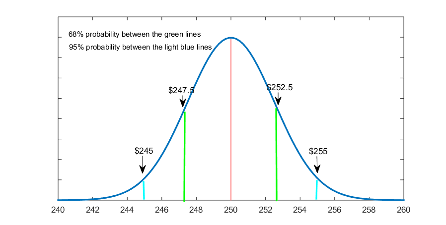
That is, we see that 68% of the sample mean prices of statistics textbooks (in hypothetical repeated sampling) would fall between $247.5 and $252.5[6] (i.e., within 1 standard error away from the mean, denoted with green in Fig. 6.1) and 95% of the sample means will fall approximately between $245 and $255[7] (i.e., within about 2 standard errors away from the mean, denoted with blue in the graph).
Since this is just a heuristic way to imagine the sampling distribution, we can restate our finding more correctly: a single, one-off sample mean will fall between $247.5 and $252.5 68 percent of the time, and between approximately $245 and $255 95 percent of the time.
Or, even more precisely, we have a 68 percent probability that the average paid price for statistics books obtained from a random sample of 1,600 students will be between $247.5 and $252.5, and a 95 percent probability that it will be approximately between $245 and $255. This means that we have a 95 percent chance that the sample mean, , will fall within $10 (i.e., ±$5) of the population mean, μ.
Quite good as far as predictions go, eh?
Of course, we rarely would have the population mean to go by, and we would never need to estimate a statistics — usually, it’s the other way around. But the sampling distribution is the same, as we still go by the CLT: With large N, it is still a normal curve. With large N, the sample mean, , is still approaching the true population mean, μ. And, with large N, the formula for the standard error is still the same, . For statistical inference, we need only follow the logic presented in Example 6.3 above (albeit in reverse).
However, there is one thing we normally do not have in order to proceed: the population standard deviation, σ. We typically use the sample standard deviation, s, as a substitute, even if this does increase the uncertainty of the estimates[8].
Then, finally, here is how inference works, in one paragraph: we use sample statistics to estimate population parameters — i.e., the statistics we calculate based on random sample data act as statistical estimators for what we truly want to know, the unknown population parameters. We do that by the postulates of the Central Limit Theorem which describe the sampling distribution, the bridge between the statistics and the parameters. By the CLT, we have the sampling distribution as normal. Again, by the CLT, we can center the sampling distribution on the sample mean, and calculate the sampling distribution’s standard error using the sample standard deviation. By applying the properties of the normal probability distribution to the sampling distribution, we then produce population estimates. Ta-da!
I will end this section with an example to illustrate the full process from the beginning to the end.
Example 6.4 Average Annual Income
Imagine you are interested in the average annual income in a medium-size city. You randomly select N=1,600 people living in that city and ask them about their annual income. You then calculate the mean of the resulting variable as $50,000, and the standard deviation as $12,000. I.e.,
 and s = 12,000
As a first guess, you could say that the average annual income in the city is $50,000. However, since we know this is an estimate, and random error exists, you can do better: you can also provide information about how certain you are about your estimate along with some margins for error.
To do that, you need to draw the sampling distribution of the mean. Following the CLT, you draw the sampling distribution as a normal curve centered on $50,000. At this point, you also need information about the sampling distribution’s dispersion, i.e., its standard error. You substitute the s you do know for the σ you don’t[9]:


Fig. 6.2 shows the resulting sampling distribution.
Figure 6.2 Average Annual Income
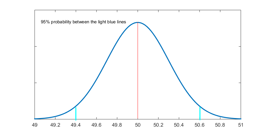
Based on the figure above (and following the same logic as in the previous Example 6.3), we find that the average annual income of the city’s population will be between $49,400 and $50,600 with 95 percent probability[10]. That is, we can be 95 percent confident that the city’s average annual income will be within $1,200 of the sample average of $50,000, or, that the city’s average annual income is $50,000 ±$600, with 95 percent certainty. (Don’t worry, all this talk of confidence and certainty will be explained in the next section.)
You should be able to appreciate that this “average annual income of $50,000 ±$600” is a much more qualified and precise statement than simply assuming the population average is the same as the sample average (which it is likely not). Now you know how much potential variability the population mean has, with a specific (and quite high!) level of certainty.
This is no way trivial, and the best “guess” you can offer as an estimate of the population mean. No other research method using sample data is able to produce a closer level of generalizability of the sample findings to the level of population, much less with the mathematical, probability-theory-backed evidence offered by random sampling. This is what statistical inference does, and now you even know how and why it works! In the next section, you can try it for yourself.
We are almost but not quite done with this abstract monster of a chapter. There is a light at the end of the tunnel — what is left is tying some loose ends, formally introducing a concept we’re already using (psst, that’s the confidence I mentioned above), and providing some final details on inference in the next section — and then we are good to go: we can start on some real research and working with variables again in Chapter 7!
- You can think of it as "the mean of the means", or the mean of the hypothetical variable mean. ↵
- After all, N is in the denominator. ↵
- On the flip side, the larger the original variables's dispersion, the larger the standard error and the smaller the original variable's dispersion, the smaller the standard error (as σ is in the numerator). ↵
- Many variables tend to be approximately normally distributed in the population. The point I'm emphasizing here is that even when they are not, the statistics of these variables based on random sample data are normally distributed. This relates to our discussion of how large N should be: if the original variable's distribution in the population is close to normal to start with, a smaller N will be fine. On the other hand, if a variable is not normally distributed in the population (or is too widely dispersed/has a lot of outliers, as reflected in σ), a relatively large N will be needed to ensure the normality of the sampling distribution. ↵
- Of course, in the video you see an approximation of a normal curve; after all, this is a finite, not infinite, number of balls. That is why the perfectly normal distribution is only a theortical concept. ↵
- That is, 250-2.5=247.5 and 250+2.5=252.5. ↵
- That is, 250-2(2.5)=250-5=245 and 250+2(2.5)=250+5=255. ↵
- We have a way to account for that, however, as we will see in Section 6.6 on the t-distribution below and the concept of degrees of freedom. ↵
- Recall that a "hat" over a symbol indicates it being estimated. ↵
- We get these bounds (i.e., within about 2 standard errors away from the mean) through 50,000-2(300)=50,000-600=47,400 and 50,000+2(300)=50,000+600=50,600. ↵