Chapter 9 Testing Associations I: Difference of Means, F-test, and χ2 Test
9.5 Between Two Discrete Variables: the χ2, Part 3
We definitely need to use the χ2 for testing contingency tables whee at least one of the variables has more than two categories, as we no longer have only two proportions to consider.
Example 9.7 Citizenship and Education, NHS 2011
A lot has been written about Canada’s selective immigration practices: the Canadian government is committed to getting “the best and the brightest” immigrants through a point system which awards more points the more education the prospective immigrant has. [CITATIONS] Be that as it may, how does the rest of the Canadian population (the one born in Canada) compare to the supposedly highly-educated foreign-born? With the help of NHS 2011 (Statistics Canada, 2019), we can find out. (Note that once again, I will use about 3 percent random sub-sample of the data, for an N=21,577.)
For this example I use the variable citizenship which has three categories: “born in Canada”, “naturalized Canadian”, and “not a Canadian citizen”. For education, I use the same recoded variable I used in Example 9.2 in Section 9.2 earlier, namely degree. Degree has six categories, ranging from (1) “no high school degree” to (6) “PhD” (for full category listing, see Example 9.2).
Table 9.4 cross-tabulates citizenship and degree in a busy-looking 3×6 table (that’s 18 cells!).
Table 9.4 Degree by Canadian Citizenship Status (NHS 2012)
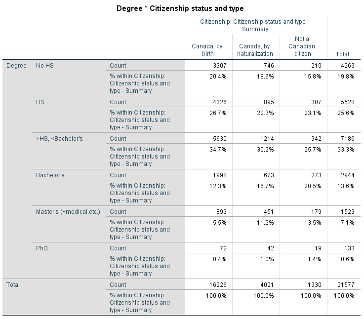
What do we see? Let’s carefully examine the evidence[1]. While all citizenship groups follow a similar vertical “spread” (i.e., relatively few people without degrees, most people with high/secondary school and some post-secondary school certificates and some sort of Bachelor’s degrees, then decreasing proportions in the higher education categories), this is not what we are interested in. Recall that we are looking for a pattern between the two variables’ categories/groups — we are comparing groups on their levels of education.
As such, we see that fewer naturalized Canadians (18.6 percent) and fewer still non-Canadian citizens (15.8 percent) have no degrees compared to Canadian citizens (20.4 percent). Furthermore, in the three highest education categories (Bachelors, Master’s, and PhD), both naturalized Canadians and non-Canadian citizens outperform those born in Canada (while the non-Canadian citizens even outperform naturalized Canadians in turn): 16.7 percent of naturalized Canadians and 20.5 percent of non-Canadian citizens have Bachelor’s degrees compared to only 12.3 percent of Canadians born in the country; 11.2 percent of naturalized Canadians and 13.5 percent of non-Canadian citizens have Master’s degrees compared to only 5.5 percent of the ones born in Canada; and, finally, 1 percent of naturalized Canadians and 1.4 percent of non-Canadian citizens have PhD’s compared to 0.4 percent of those born in Canada.
Thus, the table suggests a pattern — Canadians born elsewhere and non-Canadian citizens seem to have more education than the Canadian-born. Whether this pattern showing difference in proportions in the education degrees among the different citizenship status groups is statistically significant (i.e., generalizable to the Canadian population) remains to be checked — through a χ2–test.
These are our hypotheses:
- H0: Citizenship status and educational degree are not associated; Canadian-born, naturalized citizens, and non-Canadian citizens are on average similarly educated, and are equally likely to be highly educated.
- Ha: Citizenship status and educational degree are associated; Canadian-born, naturalized citizens, and non-Canadian citizens have different levels of education on average, and are not equally likely to be highly educated.
I would guess you would rather not calculate the expected frequencies and their differences from the observed frequencies for all 18 cells (but if you want to do it, who am I to stop you), so I’ll report the SPSS output instead.
With χ2=449.543, df=10[2], and p<0.001, we have enough evidence to reject the null hypothesis and conclude that citizenship status and educational degree are statistically significantly associated: people born in Canada, naturalized Canadians, and non-Canadian citizens differ in their levels of education. It seems indeed that Canadians born in the country are on average less educated than both naturalized Canadians and non-Canadian citizens, perhaps as a result of the selective criteria for Canadian immigration.
Important conditions for using the χ2-test. For the χ2-test to work properly, two conditions must be met: 1) the expected count should not be less than 1 for any of the contingency table cells; and 2) no more than 20 percent of the cells should have an expected count less than 5. SPSS warns you about violations of these conditions in the output; if you are not using SPSS you should make sure the conditions are met before proceeding with analysis. Either way, if these conditions are not met, you should not use the χ2-test and consider a different type of testing instead (not discussed here).
Finally, a brief word of warning.
Watch Out!! #17 . . . for Identifying The Wrong Pattern
Once again, the warning is about how to read a contingency table in light of an association between two variables. The pattern (association) in which we are interested and the one we test is a comparison between the groups of one variable on the categories of the other variable. Thus, looking at how the observations are divided within each group is only marginally relevant to the research question, and does not contribute to analyzing the association in question.
In Example 9.7 above, all immigration status groups were divided relatively similarly across the educational categories but, as interesting as you may find this “pattern”, that is not an indication of an association — comparing the percentages/proportions of the different groups in the same category is. In other words, in that example we were interested in whether there was a difference in percentages/proportions among the Canadian-born, naturalized Canadians, and non-Canadians citizens with no education, or with high school degree only, or with some college degree or certificate only, or with Bachelor’s degree, etc. We were not interested in what percentage of Canadian-born (or naturalized, or non-Canadian citizens) have no degree, and what percentage have high school degree, and what percentage have some college degree or certificate, etc. (if you recall, the latter add up to a 100 percent, and can be referred to as how the observations are spread across categories within each group).
As in Section 7.2.2, what it comes down to is knowing which way to read the table, according to the research question you have[3]. To use the language of causality, to the extent that you can identify an independent and a dependent variable, to examine an association between the variables you will be looking to compare the groups of the independent variable on the categories of the dependent variable.
We finish the chapter with the tips on using SPSS for χ2-testing.
SPSS Tip 9.3 The χ2-test
- From the Main Menu, select Analyze, and from the pull-down menu, click on Descriptive Statistics and then Crosstabs;
- From the variable list on the left, select your variable (the independent variable, with groups to be compared) and, using the bottom arrow, move it to the Column(s) empty space on the right;
- From the variable list on the left, select your variable (the dependent variable, on whose categories you will compare the groups) and, using the bottom arrow, move it to the Row(s) empty space on the right[4];
- Click on Statistics and select Chi-square at the top of the new window, click Continue;
- Once back in the Crosstabs window, click Cells; in the new window keep Observed[5] in Counts selected, and further select Column in Percentages; click Continue;
- Once back to the Crosstabs window, click OK.
- SPSS will provide the requested output in the Output window: a contingency table followed by a χ2-test table, containing the χ2-value, df, and p-value[6].
With this, we turn to our last remaining topic: the testing and investigation of the association between two continuous variables in Chapter 10, next.
- Do not forget to focus on the percentages, not the number count in each cell! Recall that you can only compare relative frequencies (relative to group size, that is). ↵
- Df=(rows-1)(columns-1)=(6-1)(3-1)=5(2)=10. ↵
- I remind you again of the rule of thumb: if the groups you are comparing are in the columns, and the percentages down the columns add to 100 percent, then look at and compare the percentages/proportions on the same row. If the groups you are comparing are in the rows, and the rows add up to 100 percent, then compare the percentages down the same column. ↵
- Again, the convention is to put the independent variable in the columns and the dependent variable in the rows. This is not a hard-set rule, however, and it is perfectly acceptable to do it the opposite way. The only thing that is not a matter of preference is for which percentages you should ask, columns or rows. If your independent variable is in the columns, you need column percentages to compare, if your independent variable is in the rows, you need row percentages to compare. In this latter case, this is a hard-set rule, and if you violate it, you will not be able to properly identify -- and test -- the association you might be investigating. ↵
- Note that from here you can also request Expected counts if you would like to check them at any point. ↵
- Note that the table contains more than just the χ2-test; discussing the rest of the tests is beyond the intended scope of this book. ↵