Chapter 10 Testing Associations II: Correlation and Regression
10.2 Basics of Linear Regression
You may find it surprising but you already have an idea about linear regression from Section 7.2.3. Again, when describing and examining the association between two continuous variables, we can use the correlation coefficient r and a scatterplot plotting the observations in a coordinate system. To visualize the linear relationship between the variables, we could also add a line of best fit to the scatterplot. The line of best fit is actually also called a regression line; and regression itself is based upon the concepts of correlation and variance, with which you are already familiar.
You might be asking yourselves at this point what regression adds to the analysis of two continuous variables, or in other words, why do we even need it — don’t we already have Pearson’s r for that? As you will see in the examples below, linear regression allows us to precisely calculate and predict a change in the dependent variable that is due to the independent variable.
What we say in this case is that the independent variable explains a percentage of the variance of the dependent variable. Think about it this way: the dependent variable varies due to arguably many causes (i.e., independent variables), which affect it to a different extent and which each explain some part of its total variance. Through linear regression, we are able to quantify to what extent an independent variable explains the variability of the dependent variable, i.e., to what extent it affects it[1]. To take the example about parental and offspring education from the previous section, doing a regression analysis on these two variables would allow us to predict how much more education a respondent is expected to have for one more year of schooling for the parent[2] (father, in our case), and what percent of respondent’s schooling is explained by the years of education of the parent.
How does linear regression do all that? To put it simply, through the regression line (of best fit), or more precisely, through the way the regression line is created.
The linear function. How do you draw a line? The simplest method requires exactly two pieces of information: a starting point of the line, and an indicator of slope (so that you know whether the line is straight, sloping upward, or sloping downward). This is captured in the following formula:
![\[y=\alpha + \beta x\]](https://pressbooks.bccampus.ca/simplestats/wp-content/ql-cache/quicklatex.com-b9ac66ac31e50212f91c42437d5cff23_l3.png "Rendered by QuickLaTeX.com")
where α is the line’s starting point and β is the slope of the line. The two variables, x and y, are the independent and the dependent variable, respectively: we know this because the formula establishes y as a function of x (i.e., if we know α and β, we can calculate y for any value of x).
Let’s take a brief example.
Example 10.2 Class Assignment Mark
Imagine you are given a written, take-home assignment in some class. Your professor has stipulated that there are three part of the assignment, each worth 30 points, and that you would receive 10 points just for turning in your work.
In this case, your assignment mark is entirely a function of your submitted work. You will be getting 10 points to start with, then 30 points for fulfilling each of the three requirements. The class grades on the submitted assignments could thus be 10 points (0 completed requirements), 40 points (1 completed requirement), 70 points (2 completed requirements), and 100 points (3 completed requirements). Figure 10.1 plots this.
Figure 10.1 Assignment Mark as a Function of Completed Requirements
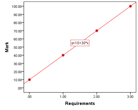
As you can see, the relationship between the two variables, assignment requirements completed and assignment mark, is simply
![\[y=10+30x\]](https://pressbooks.bccampus.ca/simplestats/wp-content/ql-cache/quicklatex.com-b99f276d438a5de736e61a943f0a7a1b_l3.png "Rendered by QuickLaTeX.com")
as helpfully shown in the graph itself. This is a summary form of having to write out all the observations:
- when x=0,

- when x=1,

- when x=2,

- when x=3,
 [3].
[3].
In the example above α=10 and β=30: the line starts at x=0 and y=10, and for each additional unit of x (i.e., each additional requirement completed), y increases by 30 points.
In fact, these are the exact definitions of α and β. That is, α is the value of y when x=0, also called Y-intercept (as it shows where the regression line crosses the vertical Y-axis), and β is the slope, also called the regression coefficient, i.e., the amount of change in the dependent variable y expected for every unit change in the independent variable x (or simply, the size of the effect of x on y).
Let’s now take a look at the regression model in detail.
- Multivariate regression thus allows for direct comparisons of the size of the independent variables' effects. In the bivariate case, we only focus on the effect of one independent variable, without considering and accounting for others -- which is not something you should do in a real-life social science research, especially in terms of causal analysis. Again, the bivariate case serves only as an illustration/introduction to the expansive topic of regression in general. ↵
- Or, to put it differently, if one father has one more year of schooling than anther father, how much more schooling the offspring of the first would be expected to have in comparison to the offspring of the second. ↵
- Of course, to draw a line you only really need two points. Thus if you only take x=0/y=10 and x=3/y=100 and connect these points with a line, the line will also pass through x=1/y=40 and x=2/y=70. This is a useful property if you need to draw a line by hand. ↵