Chapter 4 Measures of Dispersion
4.2 Interquartile Range
Unlike the range which focuses on the extreme ends, the interquartile range (frequently referred to as IQR) looks into the distribution of observations around the “centre”. To that purpose, it splits the distribution into four equal parts called quartiles (from the Latin quartus, meaning one-fourth, i.e., a quarter), and then provides the range of the middle two parts taken together. This sounds more complicated than it actually is, so let’s turn to examples and make it better.
To begin, let me first demonstrate what all this means with a set of raw values which we can call, say, hours worked per week.
Example 4.2 Weekly Hours Worked (Raw Data)
Imagine you have been hired as a research assistant (RA) on a research project. You have worked 20 weeks in total in the past two semesters, ten weeks in each semester (with your classes and all, you couldn’t work every week). The maximum hours per week you could work was 15, limited by the nature of your contract. You make a list of all hours you have worked in each of the twenty weeks, and you list the twenty values in ascending order. Here they are:
2, 3, 3, 4, 5, 7, 7, 7, 8, 8, 10, 10, 10, 10, 12, 12, 13, 13, 13, 14
If you recall from our discussion of the median, to split a group of values into equal parts we need the values’ positions in the order. You can find these in the table below:
Table 4.1 Values and Their Positions of Hours Worked per Week
| Position | Hours Worked per week | Position | Hours Worked per Week |
| (1) | 2 | (11) | 10 |
| (2) | 3 | (12) | 10 |
| (3) | 3 | (13) | 10 |
| (4) | 4 | (14) | 10 |
| (5) | 5 | (15) | 12 |
| (6) | 5 | (16) | 12 |
| (7) | 7 | (17) | 13 |
| (8) | 7 | (18) | 13 |
| (9) | 8 | (19) | 13 |
| (10) | 8 | (20) | 14 |
You might be tempted to use an intuitive method for splitting the set of twenty values given in the example into 4 equal parts (i.e., into quartiles) by simply dividing 20 by 4, which will let you have 5 values in each quartile:
2, 3, 3, 4, 5 5, 7, 7, 8, 8 10, 10, 10, 10, 12 12, 13, 13, 13, 14,
Thus the interquartile range (or “the range of the middle two parts taken together”) of the entire set of 20 values would be the range of 5, 7, 7, 8, 8, 10, 10, 10, 10, 12.
A quick-and-dirty calculation would show that the IQR is (12-5=) 7 hours. You would be correct — indeed, the interquartile range is 7 hours — but I’ll stop you nevertheless. This worked out only because I’ve chosen the numbers between the first and the second quarter of cases to be both 5, and the numbers between the third quarter and the last to be both 12. You need to read below to find out the proper method for obtaining the IQR. (The example continues further down.)
Quick-and-dirty calculations are not precise, even if they serve their purpose to give you a basic idea of what we are doing. Now that you’ve seen where this is going, let’s do everything properly.
First, we need to calculate the precise positions of the values that separate the quartiles. Recall how we used to split a set of values in two in order to get the position median. We used the following formula:
 ←“position of the median”
We’ll follow the same logic to split each of the halves in two themselves. Thus let me restate the above formula to this:
 ←“position of the median”
Since we effectively multiply N+1 by 0.5 in order to split the entire set in two halves (or, to get one half of the data), to split the first half of the values further in two itself, we need to multiply N+1 by “half of 0.5”, i.e., by 0.25 (essentially getting one quarter of the data):
 ← “position of the first quartile”
By analogy, splitting the second half in two itself will require getting three quarters of the data, or to multiply N+ 1 by “0.5 and a quarter”, i.e., by 0.75:
 ← “position of the third quartile”
If you follow the logic, you’ll easily conclude that the median is also de facto the second quartile (i.e., two quarters of the data).
To restate, we have the following way to split the data into four equal parts:
The position of the first quartile, Q1, is found through  .
.
The position of the second quartile, Q2 (a.k.a the median), is found through  .
.
The position of the third quartile, Q3, is found through  .[1]
.[1]
Now let’s use our newfound formulas in the Example 4.2.
Example 4.2 Weekly Hours Worked, Continued
With N=20, we get:
Q1‘s position → 
Q2‘s position → 
Q3‘s position → 
Once again, do not forget that all these formulas provide the positions of the quartiles, not their respective values. To see the values, we have to look at Table 4.1 above which cross-lists the cases’ positions and values. Since there is no Case #5.25, we know that the value we’re looking for is between Cases #5 and #6 (a quarter further than #5) — but as the values of both Cases #5 and #6 are 5, we conclude that the value of the first quartile is 5.
Similarly, there is no Case #15.75 (so the value we’re looking for is three quarters past the 15th case), but both Cases #15 and #16 are 12, so we conclude that the third quartile is 12.
We are still interested in the interquartile range — or the range of the two middle quarters of the data (or the middle 50 percent, so to speak). Then, since
Q3 = 12 and Q1 = 5,
we have that
Q3 – Q1 = 
Or, we have found that the IQR for hours worked per week is 7 hours per week. Or, at the mid-range, your hours worked per week varied between 5 and 12 hours per week.
Alright, but why, you might ask — couldn’t we just have the range and be done with it?
The value added of using interquartile range is that it takes care of outliers, so it’s frequently a better measure of dispersion than range. The IQR provides the spread of the centrally located 50 percent of the data which in many situations paints a more accurate picture of how “the more typical” of the variable’s cases are spread out, rather than looking at the more extreme spread provided by the range which encompasses all cases, even the clear outliers.
All in all, however, just like with choosing whether to use a median or mean, the decision which of these two measures of dispersion is the more appropriate one to be used and reported depends on the specific situation and the researcher’s discretion. I would urge you, as a beginner researcher, to make a habit of reporting both the range and the interquartile range, while simultaneously discussing the effect of any potential outliers.
Instead of working with raw data, we might have frequency tables at hand. How do we get the range and IQR from aggregated data? For the range, simply subtract the lowest value (the one listed first in the Values column, of course) from the highest value (the one listed last in the Values column) and report the difference (in its appropriate units of measurement). For the IQR, look for the 75th percentile (i.e., Q3) and the 25th percentile (i.e., Q1) in the Cumulative Percent column, then subtract the Q1 value from the Q3 value, and again report the difference. (This is similar to how we looked for the 50th percentile for the median, Q2, in Section 3.3 (https://pressbooks.bccampus.ca/simplestats/chapter/3-3-the-median-with-frequency-tables/).)
Exercise 4.1 Range and IQR for Cigarettes Smoked per Day
Practice your newly acquired skills to find Q1, Q2 (i.e., the median), and Q3 in the following table. Calculate and report the range and the interquartile range for number of cigarettes smoked each day.
Table 4.2 Number of Cigarettes Smoked Per Day by Daily Smokers (CCHS 15/16)
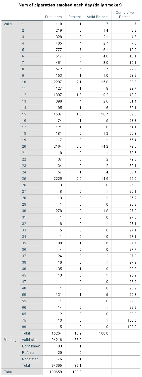
To make sure you’re doing it correctly, let’s quickly check your answers right away. The range is of course (99-1=) 98 cigarettes per day. To find the IQR, you must have first identified Q1= 10 (since 23.9 percent of the cases make up to 9 cigarettes per day, the 25th percentile falls in the 10 cigarettes per day category) and Q3 = 20 (since 65.4 percent of the cases make up to 19 cigarettes per day, the 75th percentile falls in the 20 cigarettes per day category). Then the IQR is (20-10=) 10. Thus you see the difference between range and interquartile range: while the range might leave you with the impression that cigarettes smoked per day vary by almost a hundred for daily smokers, the middle half of the cases actually only vary by 10 cigarettes.
Of course, there’s also SPSS. Check below to see how to find the range and IQR (semi-) directly.
SPSS Tip 4.1 Obtaining Range and Interquartile Range
- From the Main Menu, select Analyze, then Descriptive Statistics, and then Frequencies;
- Select your variable of choice from the list on the left and use the arrow to move it to the right side of the window;
- Click on the Statistics button on the right;
- In this new window, check Quartiles from the Percentile Values on your top left and check Range (and Minimum and Maximum if you wish) from the Dispersion section below it;
- Click Continue, then OK.
- Range (along with the smallest and largest values, if you asked for them) will be reported in the Output directly.
- To obtain the IQR, simply subtract the value reported as 25th percentile from the value reported as 75th percentile.
With the range and IQR covered, we are halfway through the typically used measures of dispersion. On to the remaining two, the variance and the standard deviation.
- Obviously, we don't speak of a fourth quartile, as four quarters comprise the whole thing: the fourth quartile would simply be 100%, or all of the data. ↵