Chapter 2 What Data Looks Like and Summarizing Data
2.1 Data Sets and What Data “Looks” Like
By now you have learned that variables are tools that allow us to measure concepts and to collect information about them. As such they are comprised of information — information that varies across the units of analysis (the ‘things’ on which we collect information, be it people, organizations, countries, etc.). So far, we have discussed individual variables – but creating and collecting information on a single variable is uncommon. Generally, we collect information on many variables at the same time (which, in turn, allows us to analyze variables together and hypothesize about possible associations between variables).
Variables “live” in data sets (or datasets, as I prefer; both usages are common). A dataset is a collection of variables that lists the information (or observations) gathered on them from the units of analysis. As usual, I focus on analysis of people for simplicity’s sake (but do keep in mind the units of analysis can be something else.)
The best way to visualize a dataset is as a sort of a table (a.k.a a matrix) which summarizes the responses from every individual (in the rows of the table) on the variables in the dataset (in the columns of the table). As such, the size of a dataset depends on two things: the number of variables and the number of individuals supplying information (a.k.a. respondents). Typically, datasets vary in size from just a handful of variables and few respondents to hundreds of variables and thousands of respondents. (Huge datasets — comprising information on millions of people — exist too; these are known as big data. Big data is not analyzed in the conventional ways regular datasets are, so from now on we’ll leave big data aside as it’s not the subject of this book.)
To start small, imagine you have just four friends at your university and you decide to list some items of information about them (say, maybe you want to compare your standing at the university with theirs, and to see differences and commonalities between you and them). You could do that in a sentence form, for example, thus: Arjun, who is twenty years old, speaks Punjabi at home and is a first year student in the Business School, has a job and his GPA is 3.6. Benjamin, on the other hand, who is 25, speaks German at home and is a third year Science student, also has a job but his GPA is lower than Arjun’s at 3.2. Cecilia, who speaks Spanish at home and is a fourth year Health Sciences student doesn’t have a paying job and her GPA is the highest of your friends, 4.0. Finally, Xingxing is also a first year student and is employed like Arjun but she is an Arts major, speaks Mandarin at home, and her GPA is 3.3.
Indeed, you might do that but the points of comparison might get lost as they are not easy to see: one has to read very carefully to keep track of who does what and has a GPA of how much. Instead, you could present the same information as it is in the table in Example 2.1 below.
Example 2.1 (A) A Hypothetical Dataset of Four Friends’s Characteristics
| Age | Year at university | Employment | GPA | Major (by Faculty) | Language spoken at home | |
| Arjun | 20 | 1 | yes | 3.6 | Business | Punjabi |
| Benjamin | 25 | 3 | yes | 3.2 | Science | German |
| Cecilia | 22 | 4 | no | 4.0 | Health | Spanish |
| Xingxing | 19 | 1 | yes | 3.3 | Arts | Mandarin |
If you do that, what you have created is a dataset. Now imagine that instead of this contrived combination of four friends and their varying characteristics, I generalize the example like so:
Example 2.1 (B) A Hypothetical Dataset of Four Individuals and Six Variables
| Variable 1 | Variable 2 | Variable 3 | Variable 4 | Variable 5 | Variable 6 | |
| Respondent #1 | Response1.1 | Response2.1 | Response3.1 | Response4.1 | Response5.1 | Response6.1 |
| Respondent #2 | Response1.2 | Response2.2 | Response3.2 | Response4.2 | Response5.2 | Response6.2 |
| Respondent #3 | Response1.3 | Response2.3 | Response3.3 | Response4.3 | Response5.3 | Response6.3 |
| Respondent #4 | Response1.4 | Response2.4 | Response3.4 | Response4.4 | Response5.4 | Response6.4 |
In Example 2.1 (B), the respondents are the four people on whose varying characteristics we have information, and these are represented by the six variables. This, however, seems rather cumbersome. Instead of “Variable 3”, and “Respondent 5”, and “Response4.3“, etc., a simpler way to represent all of these in a generalized way is through mathematical notation.[1]
So, prepare yourselves! Here comes notation:
Example 2.1 (C) A Hypothetical Dataset of Four Individuals and Six Variables 2.0
| X1 | X2 | X3 | X4 | X5 | X6 | |
| I1 | x11 | x21 | x31 | x41 | x51 | x61 |
| I2 | x12 | x22 | x32 | x42 | x52 | x62 |
| I3 | x13 | x23 | x33 | x43 | x53 | x63 |
| I4 | x14 | x24 | x34 | x44 | x54 | x64 |
In Example 2.1 (C), I1, I2, I3, and I4 are the four individuals; X1, X2, X3, X4, X5, and X6 are the six variables; and x11, x12, etc. stand for any specific characteristic/response a respondent has on a variable. More specifically, x53, for example, is the characteristic that Respondent #3 has on Variable 5. Scrolling up to Example 2.1 (A) will allow you to see that x53 is Health, which is Cecilia’s Major by Faculty.
Do It! 2.1 Reading Points of Information
In a similar vein, look up x22, x34, and x61. It’s a simple and easy task but it will help you connect notation to what it stands for, and to understand the logic underlying the way information is presented in datasets.
From here, it’s not difficult to extrapolate the specific dataset we had above to a general one. Thus, Example 2.1 (D) below presents a template of a typical dataset.
Example 2.1 (D) A Hypothetical Dataset of N Individuals and K Variables
| X1 | X2 | X3 | X4 | X5 | X6 | X7 | … | XK | |
| I1 | x11 | x21 | x31 | x41 | x51 | x61 | x71 | … | xk1 |
| I2 | x12 | x22 | x32 | x42 | x52 | x62 | x72 | … | xk2 |
| I3 | x13 | x23 | x33 | x43 | x53 | x63 | x73 | … | xk3 |
| I4 | x14 | x24 | x34 | x44 | x54 | x64 | x74 | … | xk4 |
| I5 | x15 | x25 | x35 | x45 | x55 | x65 | x75 | … | xk5 |
| I6 | x16 | x26 | x36 | x46 | x56 | x66 | x76 | … | xk6 |
| I7 | x17 | x27 | x37 | x47 | x57 | x67 | x77 | … | xk7 |
| … | … | … | … | … | … | … | … | … | … |
| IN | x1n | x2n | x3n | x4n | x5n | x6n | x7n | … | xkn |
N = number of elements in the dataset
K = number of variables in the dataset
In the table above, you may think of N as the last row on the table, i.e., the last individual for whom we have information and you may think of K as the last column on the table, i.e., the last variable we have in the dataset. Both numbers can theoretically be “any positive number”, though in practice the former is usually a number up to several thousands and the latter a number up to few hundreds. The ellipses in the next-to-last row and the next-to-last column indicate that the table is truncated: there are omitted rows between the seventh and the last individuals (i.e., between I7 and IN), and omitted columns between the seventh and the last variables (i.e., between X7 and XK). (They obviously have to be omitted so that the table can fit on the page.)
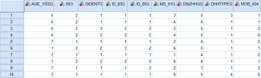
Armed with this knowledge, let’s take a look at an excerpt from a real dataset. The following Example 2.1 (E) provides a snapshot of the first ten respondents and first nine variables in the Aboriginal Peoples Survey 2012 dataset (or APS 2012 for short)[2] using a software called IBM® Statistical Package for the Social Sciences, commonly referred to as SPSS.
Example 2.1 (E) A Snapshot of Survey Data (APS 2012)
Snapshot of APS 2012‘s Data View in SPSS:
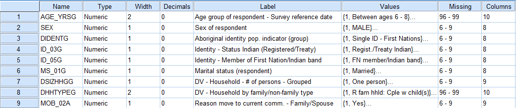
Snapshot of APS 2012‘s Variable View in SPSS:
Do It! 2.2 Understanding How Datasets Are Organized
Make sure you can connect the data snapshots from the example above with your understanding of how datasets are organized. What do the numbers in the first (blue) columns in both images represent? (Hint: this is not a variable!) What is listed in the first (blue) row in the top image? In the top image what does 1 stand for in the first white row in column ID_03G? How about the 1 in the fifth row in the SEX column?
Answer: Registered/Status Indian and male, respectively.
One thing you might find surprising is the obvious fact that all cell entries (i.e., the observations we have) are listed in a number format. Does that mean that all variables in this particular dataset are interval or ratio? What about any nominal or ordinal variables – do they not exist in this dataset? The answer is no on both accounts: the variable SEX (i.e., “Sex of respondent” as stated in Variable View) is nominal and the variable AGE_YRSG (i.e., “Age group of respondent…”) is ordinal because of the hierarchical arrangement of the responses. However, the dataset cells contain only numbers because statistical software can only analyze numerical data.
To that effect, nominal and ordinal variables appear “in code” in datasets; i.e., the categories of nominal and ordinal variables are assigned numerical values as labels to represent them in the actual dataset you might be working with. Thus, the numbers in nominal and ordinal variables’ columns are not actual numbers, they are artificially (and in the case of nominal variables, somewhat arbitrarily) assigned to represent the words contained in the categories in order to make computer-based statistical analysis possible. (On the other hand, interval/ratio variables’ categories contain actual numbers. Of course, the trick then is to learn to differentiate the actual numbers from the code/ number values used as labels in the cells of a dataset.)
Therefore, you should always keep track of the code (see the Watch Out! panel below for tips on Variable View in SPSS which allows you to do that), and remember to refer to the categories by their proper (word-based) names — not by the artificial numerical values (i.e., code) representing them!
Watch Out! #2 …for Making Hasty Decisions about Variables Based Only on Data View or Only on Variable View
It’s tempting, but you cannot deduce all categories of a variable with any certainty just by looking at the snapshot in Example 2.1 (E). You cannot do that even if, instead of a snapshot, you had the real, interactive Data View window in SPSS in front of you. Not only you might not be able to scroll through all the data (depending on its size) but, more importantly, not all characteristics might exist among the individuals. (For example, imagine the variable hair colour, and say, not one respondent having red hair: then a response “red” would not be visible in Data View, even if such a category existed in the variable.) For the same reasons you should also not decide a variable’s level of measurement based on Data View. (Remember, all data in the cells appears in numerical format, regardless if it’s an actual number or just a value label/code!)
To explore any dataset you might end up working with and all the variables contained therein, you should always look to explore not only the Data View but the Variable View of the dataset as well (in SPSS you can toggle between Data View and Variable View easily with a click of the mouse). The Variable View lists all variables along with some information about them — including something which looks like their level of measurement, called Measure (it is not included in the bottom snapshot above). The Measure information can be quite misleading for students so: Never trust this software-generated conclusion!
Instead, you should always explore both Variable View and Data View. You should note the variables’ respective categories (in Variable View, where you can click on any cell in the Values column for a full category listing) and the type of the observations you have in the cells in the table (in Data View). Then –and only then — reach the appropriate conclusion about the levels of measurement of the variables you have at hand.
What should guide your decision about a variable’s level of measurement is what you see in the Values column in Data View. To repeat, clicking on the respective column will open up a window displaying the (nominal or ordinal) variable’s categories/values along with the number label representing them in the dataset.
Again, note that reporting on the variable should be done by using its categories/values, never by the number label you see in Variable View standing in for them! This point will become more relevant and less abstract once we start learning what to do with variables, in Chapter 3.
- A note on mathematical notation, about which, I know, many students feel quite anxious: think of notation as a type of shorthand, or a sort of simplified foreign language. It's used to simplify what you can write out in words and sentences but would be too long and not as clear. The key to notation, just like with any foreign language, is to know what the symbols mean. Keep their meaning in mind, and you can read notation as fast and as easily as your own language. ↵
- APS 2012 is a Statistics Canada dataset which I will formally introduce in Ch. XX. ↵