30 Tutorial: Cyclic dominance
Introduction
Surviving in the ocean is living in a state of fear; fear of being eaten by birds, mammals and other fish. For the marine predator, it does not really matter what it consumes as long as the prey is about the right size. From this perspective, the Fraser River sockeye salmon is like many other species — an inviting mouthful swimming in the open water masses of lakes and the ocean.
Sockeye salmon are repeatedly faced with making strategic choices throughout their life cycle. They can hide and limit risk of predation, but feed little and grow slowly—or they can stay in the open and risk being eaten, but feed a lot and grow quickly. It is a constant tradeoff where they are damned if they do and damned if they don’t. Sockeye salmon, like other fish, have successfully dealt with this dilemma through evolutionary time by developing a complicated life history that includes moving between ranges of habitats varying in the risks they represent. Minimizing predation forms an important part of this strategy.
Spawning in nutrient-poor streams and moving down to lakes below the streams has been an important part of the life-history strategy of sockeye salmon because neither of these habitats can maintain year-round predator populations that are abundant enough to severely impact varying numbers of sockeye salmon. A similar strategy may be at play for the larger sockeye in the open blue water ocean — where fish can hide at depth from predators during day, and feed at shallower depths from dawn to dusk under the cover of darkness. Between the lakes and the open ocean lies a dangerous stretch through the Fraser River and the Strait of Georgia, and along the British Columbia coast to Alaska. Predators are likely to gather to prey upon the ample and seasonal supply of outward bound and returning sockeye salmon. Making it through the gauntlet likely depends upon the size and speed of the migrating sockeye, the feeding conditions they encounter — and the species and numbers of predators that seek to eat them.
Dominance cycles: role of predation?
The runs of several populations of sockeye salmon in the Fraser River system have in known history shown a four-year cycle with a dominant run, followed by a less abundant sub-dominant year class, and then two “off” years with very low abundance[1] – see Figure 1 for trends since Ricker’s paper. Larkin[2] described how this pattern can be derived in a model where predation is insufficient to influence the dominant year, but where this leads to a predator increase, which in turn has a strong impact on the following three years.
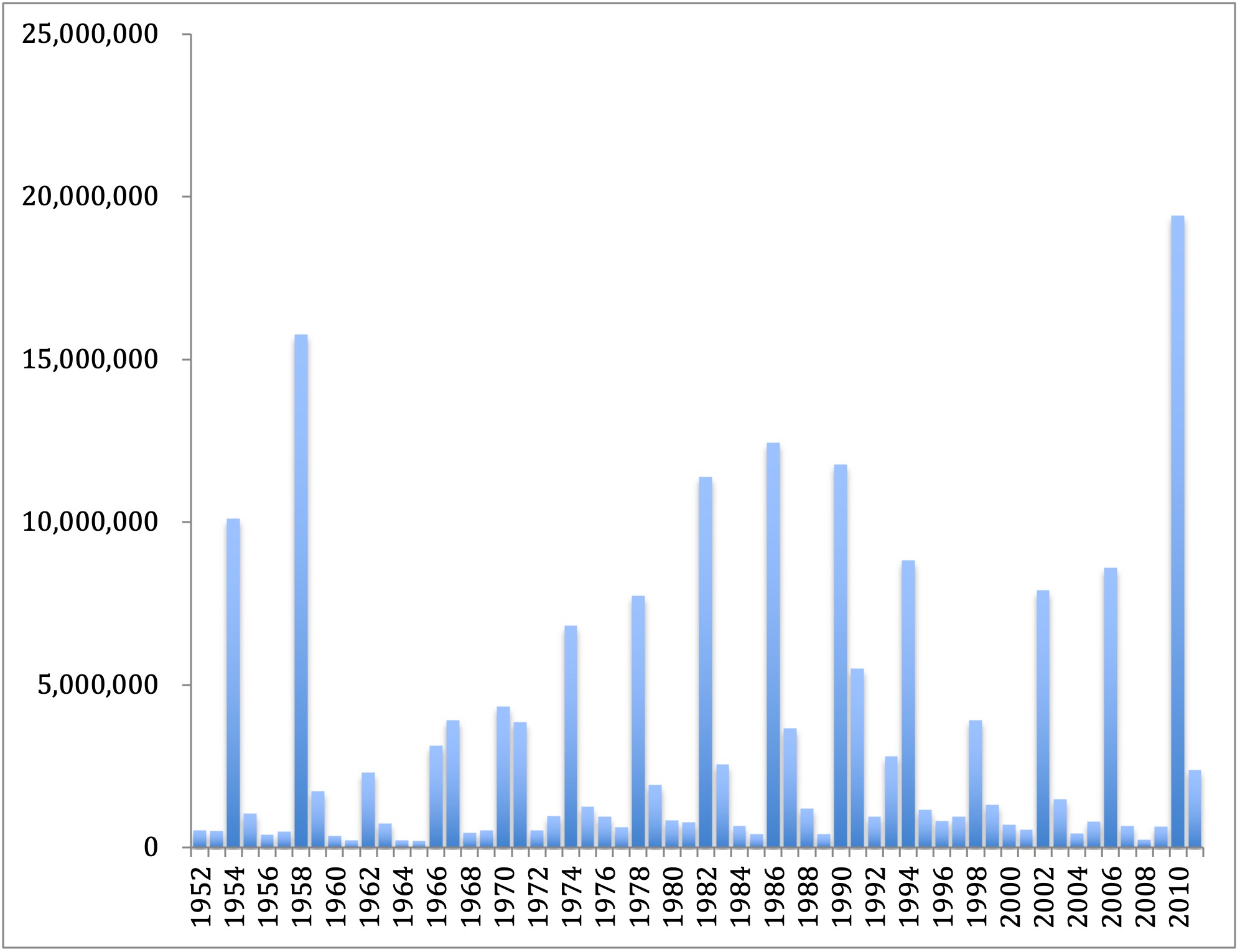
Figure 1. Estimated total run size for late summer Fraser River sockeye salmon.
Considerable work has since the 1950s taken place through the International Pacific Salmon Fisheries Commission (IPSFC) seeking to identify the cause or causes of the dominance of one brood year over others―but no clear answer is evident[3] Interestingly, IPSFC scientists in the 1950s believed that kokanee were responsible for the weak cycles because of competition for the same food, zooplankton.[4]
The incentives for building the “off” years is high,[5] but there is no indication that this is possible. It does indeed seem likely that there are inherent factors experienced by Fraser River sockeye salmon that induce the cyclic trends, which are not common elsewhere. Levy and Wood,[6] reviewed the alternative hypotheses for cyclic dominance in the Fraser River sockeye populations, and concluded that only those that involve genetic effects on age at maturation, or on disease or parasite resistance, or involved depensatory predation soon after fry emergence, seem to have merit.
Modeling cyclic dominance
Where it has been a challenge to understand why some Fraser River sockeye salmon show cyclic dominance, there has been some progress in recent years to explain the phenomenon through modeling. A German modeling group has thus been able to replicate the cyclic behaviour based on a simple three-level ecosystem model with a predator (rainbow trout), juvenile sockeye, and with zooplankton as prey.[7] They further have found that the cyclic dominance is robust to noise,[8] and that the effect is due to impacts in the nutrient poor lakes rather than in the ocean.[9] Indeed, it is only in nutrient poor lakes of the Fraser River that cyclic dominance occur, not in the nutrient rich lakes where there are sufficient competitors, and not in the ultra nutrient poor lakes where there isn’t enough productivity to support sizeable sockeye populations. The modeling also indicates that two factors are important for cyclic dominance, (1) that the carrying capacity for the prey, zooplankton, depends on the number of spawners the previous fall as their carcasses add marine-derived nutrients to the nursery lakes – spawning takes place just above such lakes, and (2) that most of the dominant year class return as four year old fish and some as five year old (as is actually the case – and some actually also as three year old). Further, the group has found that introduction in the rearing lake of a competitor to the sockeye can lead to the disappearance of the cyclic dominance unless the competitor has very low abundance.[10]
Building a sockeye model
The purpose of this exercise is to explore some basic features of predator-prey interactions that may be of relevance for understanding cyclic dominance in Fraser River sockeye salmon.
We will construct a simple ecosystem model as an Ecopath mass-balance model to describe the life cycle of Fraser River sockeye salmon, then parameterize and explore how this model behaves in the time-dynamic Ecosim module of the Ecopath with Ecosim (EwE) approach and software. See the flowchart of the model in Figure 2.
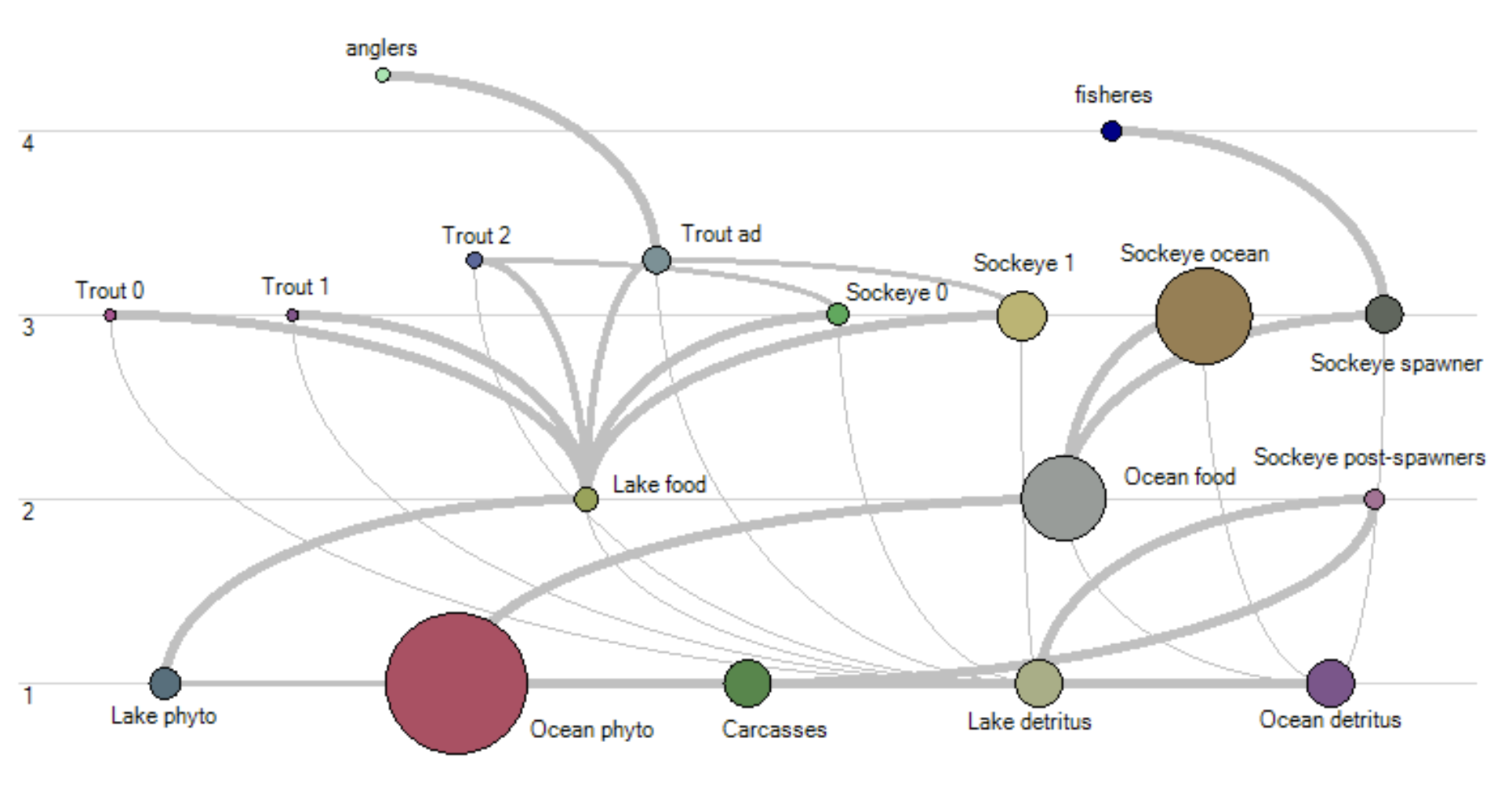
Figure 2. Flow chart for Fraser River sockeye salmon Ecopath model. The groups are arranged after trophic levels on the Y-axis, and the trout group is split in age-stance (0-years, 1 years, 2 years, and 3 years and older) and the sockeye salmon in 0- and 1-year old, which both live in the lake, an ocean stage, the spawners which returns, and the senescent post-spawners, which adds nutrients to the lake (detritus group). The size of the groups indicates biomasses – think of them as three-dimensional spheres, then the volume is proportional to biomass.
To construct the model, do as follows. Start by opening EwE6, select File > New model from the top menu. Browse to your preferred file location, and enter a name for the model. For instance, “Fraser Sockeye”. Now navigate on the Navigator (left panel) to Input data > Basic input. The model will have one group, Detritus. All models must have a detritus group, so we have entered it for you. Why? We need to be sure there is a group where we can send excreted and egested material as well as dead organism. By default they go to the detritus group.
On the Ecopath > Input > Basic input form, select Define groups (also available from the menu on top: Ecopath > Define groups). Click Edit > Insert on the right side of the form that pops up, repetitively till you have 16 groups. Then enter the group names, as in Figure 3. When you have entered all, click the Producer check mark in the Lake phyto and Ocean photo rows. On the right panel, you may also want to click the Colours > Alternate all or Random all, to get a better distribution of group colours. Click OK.

Figure 3. Ecopath > Input > Basic input > Define groups form. When entering the multi-stanza enter, e.g., Trout for one of the stanzas, then select Trout from the drop-down list.
We have a Carcasses group, that one is for post-spawning sockeye salmon, and we need to tell the model what happens to the dead sockeye – they provide nutrients (especially phosphorus, which is the limiting nutrient for primary production in the nutrient poor sockeye lakes). Select Ecopath > Input data > Detritus fate, and set the detritus fate for Sockeye post-spawners to go Carcasses. Set the detritus fate for Carcasses to go to Detritus. Save your model.
We also need to define our fishing fleets at Ecopath > Input > Fishery > Fleets, and then Define fleets above the spreadsheet and insert two fleets: anglers and fishers. We can enter catches while we are here, Ecopath > Input > Fishery > Landings. Set the angler catch of Trout adult to 0.08 t km-2 year-1, and for fishers to 0.2 t km-2 year-1 of Sockeye spawners.
Next is Ecopath > Input > Basic input, where you first need enter the basic input values from Table 1. You should be able to cut and paste from the figure (with Ctrl-C and Ctrl-V).
Table 1. Basic input parameters for groups with biomass dynamics.
| No | Group name | Biomass | P/B | Q/B | EE |
|---|---|---|---|---|---|
| 10 | Lake food | 20 | 80 | 0.995 | |
| 11 | Ocean food | 3 | 20 | 80 | |
| 12 | Lake phyto | 0.5 | 100 | ||
| 13 | Ocean phyto | 10 | 100 | ||
| 14 | Carcasses | 1 | |||
| 15 | Lake detritus | 1 | |||
| 16 | Ocean detritus | 1 |
Our model has multi-stanza groups for trout and for sockeye salmon. For these two groups we will make an age-structured model, where Ecosim will keep track of multi-cohorts for each group. The stanzas can have different diets and fisheries, as well as other input parameters. It is necessary to enter a mortality rate (Z, year-1) for all stanzas, and a “leading” biomass (B, t km-2 = g m-2) and consumption/biomass ratio (Q/B, year-1) for only one ("leading") of the stanzas. B and Q/B does not need to be for the same stanza). Ecosim then calculates B and Q/B for the other stanzas based on von Bertalanffy growth. Save your model regularly.
For the multi-stanza groups, we need to enter the parameters in Figure 4 for trout and in Figure 5 for sockeye salmon at Ecopath > Basic input > Edit multi-stanza (next to the baby pram above the Basic input form).
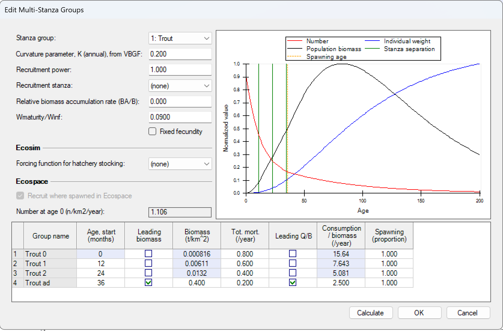
Figure 4. Multi-stanza input form for Trout.
Notice in in Figure 4, how Ecosim develops a population dynamics model for trout. The red line (declining exponentially) shows the number of individuals by monthly age, the blue line shows individual weight (increasing asymptotically), and the product of the two (black line with intermediate peak) represents the population biomass. The three vertical lines indicate the separation between the three age stanza groups.
As discussed, one of groups have to be “leading” for biomass, for trout that is the adult trout group, and one leading for Q/B, also adult trout here. The total mortality rate (Z, year-1, corresponds to P/B for biomass dynamics groups) must be entered for all stanza groups. Save your model.
Figure 5. Multi-stanza input form for sockeye salmon.
We also need to define the predator-prey linkages, and this is done on the Ecopath > Basic input > Diet composition tab. Diets are entered as proportions (based on volume or weight, preferably) and thus sum to 1 for each predator (entered by columns).
Table 2. Diet composition for the Fraser River sockeye model. Predator diets are listed by column, and are entered as proportions that sum to 1. Notice that the first 7 groups have no predators in this model. Import is food taken outside the system, e.g., by birds feeding on land. Sockeye post-spawners do not feed, but Ecopath doesn’t know how to handle that, so we’ve made them eat detritus.
| Prey \ predator | 1 | 2 | 3 | 4 | 5 | 6 | 7 | 8 | 9 | 10 | 11 | |
|---|---|---|---|---|---|---|---|---|---|---|---|---|
| 1 | Trout 0 | 0 | 0 | 0 | 0 | 0 | 0 | 0 | 0 | 0 | 0 | 0 |
| 2 | Trout 1 | 0 | 0 | 0 | 0 | 0 | 0 | 0 | 0 | 0 | 0 | 0 |
| 3 | Trout 2 | 0 | 0 | 0 | 0 | 0 | 0 | 0 | 0 | 0 | 0 | 0 |
| 4 | Trout ad | 0 | 0 | 0 | 0 | 0 | 0 | 0 | 0 | 0 | 0 | 0 |
| 5 | Sockeye 0 | 0 | 0 | 0.3 | 0 | 0 | 0 | 0 | 0 | 0 | 0 | 0 |
| 6 | Sockeye 1 | 0 | 0 | 0 | 0.3 | 0 | 0 | 0 | 0 | 0 | 0 | 0 |
| 7 | Sockeye ocean | 0 | 0 | 0 | 0 | 0 | 0 | 0 | 0 | 0 | 0 | 0 |
| 8 | Sockeye spawner | 0 | 0 | 0 | 0 | 0 | 0 | 0 | 0 | 0 | 0 | 0 |
| 9 | Sockeye post-spawners | 0 | 0 | 0 | 0 | 0 | 0 | 0 | 0 | 0 | 0 | 0 |
| 10 | Lake food | 1 | 1 | 0.7 | 0.7 | 1 | 1 | 0 | 0 | 0 | 0 | 0 |
| 11 | Ocean food | 0 | 0 | 0 | 0 | 0 | 0 | 1 | 1 | 0 | 0 | 0 |
| 12 | Lake phyto | 0 | 0 | 0 | 0 | 0 | 0 | 0 | 0 | 0 | 1 | 0 |
| 13 | Ocean phyto | 0 | 0 | 0 | 0 | 0 | 0 | 0 | 0 | 0 | 0 | 1 |
| 14 | Carcasses | 0 | 0 | 0 | 0 | 0 | 0 | 0 | 0 | 0 | 0 | 0 |
| 15 | Lake detritus | 0 | 0 | 0 | 0 | 0 | 0 | 0 | 0 | 1 | 0 | 0 |
| 16 | Ocean detritus | 0 | 0 | 0 | 0 | 0 | 0 | 0 | 0 | 0 | 0 | 0 |
We also need to define what happens to the detritus that is produced in the system. For this we set the Input data, Detritus fate as in Figure 6.
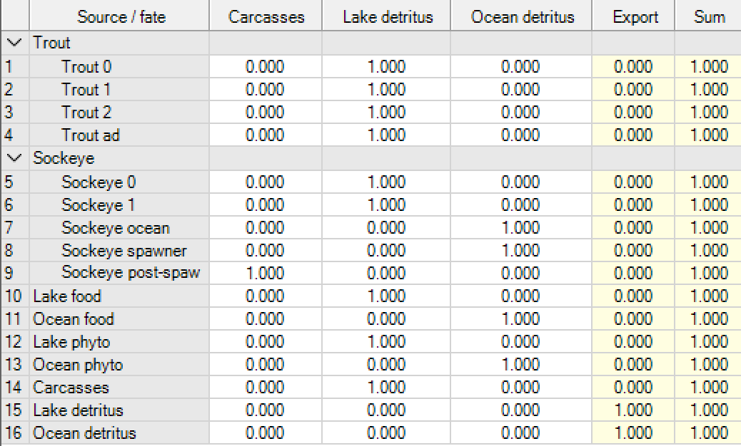
Figure 6. Detritus fate for the groups in the sockeye model.
We now have all the input parameters we need for the Ecopath model, so save the model, and let Ecopath mass-balance the model. For this, click Ecopath > Output > Basic estimates, where you may get a warning about respiration, which you can ignore. The warning is for the sockeye post-spawners where Z >> Q/B, which gives a negative respiration, (Respiration = consumption – production – unassimilated food). Ecopath assumes production = mortality, which causes this, and the message can just be ignored (if it shows up).
Next, check for mass balance, Ecopath > Output > Basic estimates to get an output form where the values that Ecopath has estimated are shown with blue font. For this model that is EE for all groups, apart from for lake food where biomass (B) was estimated. If you have entered the input parameters correctly, the model should balance. If not, check the Mass-balance chapter for guidelines.
Time dynamics
It’s time to load Ecosim, Ecosim > Input > Ecosim parameters. You’ll be asked to create a scenario – which will hold all the information that is needed to save a run – you can have many scenarios within one model. Any name will do.
The sockeye rearing lakes are nutrient poor, and we will make a few changes to the default parameter setup to start considering this. On Ecosim > Input > Ecosim parameters, set Duration of simulation (years) to 40 years, and change the Base proportion of free nutrients to 0.1. The last parameter will tell Ecosim that most of the nutrients will be bound in living matters and detritus (including sockeye salmon carcasses), and that it is with the decomposition of those that much of the nutrients will be recycled/added.
Assumptions about carrying capacity will also impact the results, to explore aspects of this go to Ecosim > Input > Vulnerabilities, and change the vulnerability multipliers for the groups 1 to 6 (trout and sockeye salmon's lake stages) to 1 (by column, not row), which makes these groups be dependent on prey production (bottom-up control). For the sockeye salmon ocean stages (groups 7 and 8), to 5, also by column, not row. This is telling Ecosim, that if the sockeye salmon in the ocean are somewhat far from their carrying capacity, and will be able to increase the predation mortality the cause on their prey up to 5 times compared to the baseline Ecopath consumption.
Now it is time to make a run, go to Click Time dynamic (Ecosim), Output, Run Ecosim, and click the Run button in the lower right corner. Ecosim will then make a 50-year run and display the results (Figure 7).
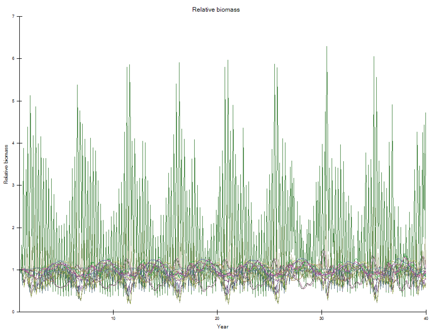
Figure 7. Relative biomasses in Ecosim after initial run. The most diverging group is (sockeye) carcasses, which has 9 cycles over the 40 year simulation. So, a cycle of just over 4 years.
The graph shows relative biomasses over time (so Ecosim biomass / Ecopath biomass). Notice from the run that sockeye will become cyclic after a few years. The periodicity is slightly larger than 4 years, which is about what is observed for Fraser River sockeye salmon.
So the status is that we've been able to create a simple model that shows cyclic dominance quite similar to what is observed. This does of course not mean that we've found the right mechanism for why the cycle occur, but we've shown that it could possibly be because of combined predation and competition interaction with the dominant piscivore in the lakes, rainbow trout.
The model is (relatively) simple and there are lots of mechanisms not considered. We could for instance let sockeye salmon only spawn for a couple of months seasonally. If we just introduce that (Ecosim > Input > Egg production), the cyclic dominance will go away. Why? Likely because we've introduced seasonality on this one aspect only, not throughout – it's as Carl says: one can't be a bit pregnant, if you introduce seasonality it's all the way through.
So, the model is good enough to demonstrate that a potential cause is feasible, it can certainly be improved (feel free to give it a go), but as interesting is: are there other potential mechanisms that may be causing the cyclical patterns of Fraser River sockeye salmon? If you have ideas: make a simple model to check it.
You can download the sockeye salmon EwE database from this link.
- Ricker, W., 1950. Cycle dominance among the Fraser sockeye. Ecology 6–26. ↵
- Larkin, P., 1971. Simulation studies of the Adams River sockeye (Onchorhynchus nerka). Canadian Journal of Fisheries and Aquatic Sciences 28, 1493–1502 ↵
- Hume, J.M.B., Shortreed, K.S., Morton, K.F., 1996. Juvenile sockeye rearing capacity of three lakes in the Fraser River system. Canadian Journal of Fisheries and Aquatic Sciences 53, 719–733. ↵
- Sebastian, D.C., Dolighan, R., Andrusak, H., Hume, J., Woodruff, P., Scholten, G., 2003. Summary of Quesnel Lake kokanee and rainbow trout biology with reference to sockeye salmon, Stock Management Report No 17. Province of British Columbia. ↵
- Walters, C.J., Staley, M.J., 1987. Evidence against the existence of cyclic dominance in Fraser River sockeye salmon (Oncorhynchus nerka), in: Smith, H.D., Margolis, L., Wood, C.C. (Eds.), Sockeye Salmon (Oncorhynchus Nerka) Population Biology and Future Management. Canadian Special Publication of Fisheries and Aquatic Science, 96, pp. 373–384. ↵
- Levy, D.A., Wood, C.C., 1992. Review of proposed mechanisms for sockeye salmon population cycles in the fraser river. Bulletin of Mathematical Biology 54, 241–261. ↵
- Guill, C., Drossel, B., Just, W., Carmack, E., 2011. Journal of Theoretical Biology. Journal of Theoretical Biology 276, 16–21. doi:10.1016/j.jtbi.2011.01.036 ↵
- Schmitt, C.K., Guill, C., Drossel, B., 2012. The robustness of cyclic dominance under random fluctuations. Journal of Theoretical Biology 308, 79–87. doi:10.1016/j.jtbi.2012.05.028 ↵
- Guill, C., Carmack, E., Drossel, B., Post, J., 2014. Exploring cyclic dominance of sockeye salmon with a predator–prey model. Canadian Journal of Fisheries and Aquatic Sciences 71, 959–972. doi:10.1139/cjfas-2013-0441 ↵
- Schmitt, C.K., Guill, C., Carmack, E., Drossel, B., 2014. Effect of introducing a competitor on cyclic dominance of sockeye salmon. Journal of Theoretical Biology 360, 13–20. doi:10.1016/j.jtbi.2014.06.021 ↵
