48 Spatial modelling primer

This chapter gives a primer about some of the higher level questions that are dealt with in connection with spatial modelling in EwE.

When to “go spatial”?

So, you’ve created an ecosystem model, tuned it with regard to carrying capacity in order to replicate the known ecosystem history, and you’re considering taking it to the next level, to explicitly represent spatial patterns and dynamics. When should you do that?  The first and foremost question to consider is whether the policy/research question (see chapter) that is driving your work is inherently spatial. If it is, consider constructing a spatially-explicit model. Take for instance if you’re to evaluate the impact of a marine protected area (MPA) – such a question indeed calls for a spatial model.

EwE includes a spatial model, Ecospace, which in essence provides an model with a bunch of Ecosim models, each running in a cell in a regular spatial grid, while keeping track of flows between spatial cells along with human and environmental impacts.  The Ecospace model was originally^[1] developed to address questions about the functioning of MPAs, but has has over the years been expanded in various ways to become a capable tool for ecosystem-based fisheries management (EBFM), multi-sectoral EBM, and prediction of climate change impacts. The details of that are described in the current and next part of this textbook.

It should be stressed, once again, that Ecospace is not “better” than Ecosim, which in turn is not “better” than Ecopath. Ecospace is more complex, and as a general rule, the best model to address a given policy/research question is the simplest model that can address it. Adding more “realism” may not improve a models predictive capability, it may have the opposite effect, indeed.  So, you “go spatial” when there’s no way around it, when you really need it. Not in order to produce pretty maps –and yes, we all love pretty maps, but that’s not a sufficient reason for adding complexity).

Eulerian vs. Lagrangian movement

There are two basic approaches to modelling spatial movement (at least in fluid dynamics, which we can lean heavily on for modelling trophic flows), Eulerian vs. Lagrangian, (Figure 1).

Eulerian^[2] approaches analyzes overall flow patterns over space and time 
from the fixed viewpoints of spatial cells, and estimates movements across cell boundaries, averaging the flows in and out of cells.  This form for modelling goes hand in hand with population-based modelling where the basic unit is the population, which in turn in impacted by changes in the form of flows, e.g., mortalities. The original (and default) Ecospace model representation is an example of a Eulerian approach.

Lagrangian^[3] approaches in contrast tracks the movement of individuals in a system 
and follows their trajectories over space and time.  Given that the Lagrangian approach opens for following individuals, it serves as a foundation for Individual Based Models (IBM), also known as agent-based models, which models populations with all (or representative) individuals modelled explicitly.

For EwE multi-stanza groups, you have the option of using the default Eulerian or an IBM approach in Ecospace (see chapter).

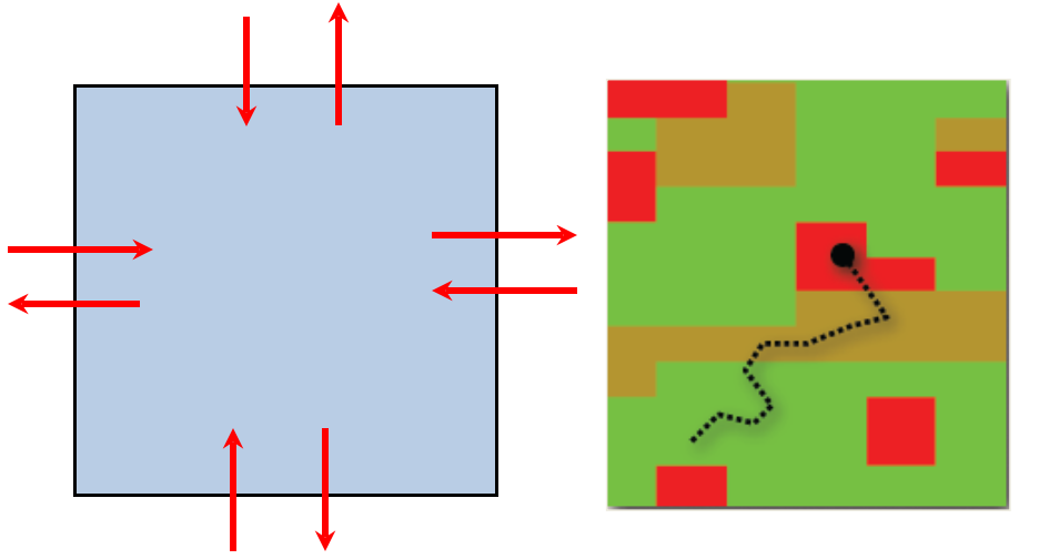
Figure 1. Eulerian (left) vs. Lagrangian (right) approaches to modelling of spatial movements. Eulerian approaches average flows from a fixed perspective, here a spatial cell where it keeps track of movements and advection to the four neighbouring calls. Lagrangian approaches track particle flows spatially across the model domain. 

Domain definition

Spatial extent

There are several questions to be addressed as part of the model domain definition. A first is the spatial extent of the model. The key factor here is that your model policy/research question should dictate the model extent. That may not seem very specific, indeed it isn’t, so let’s illustrate with an example.

If you’re working on fisheries management in the Azores Islands where both seamount and pelagic fisheries are important, you’ll make a local model that includes all of the relevant fisheries.  This will then include tuna species whose distribution and population dynamics is at the scale of the North Atlantic. How do you deal with that?  The simple way is to include immigration and emigration for the tuna. This will result in the given amount of tuna always coming in (immigration), while the amount of tuna leaving (emigration) will be a function of how many that are caught in the Azores area.  This will not be correct, but from the point of view of the Azores Islands’ managers, it is a reasonable assumption^[4].

Still, it will not capture the dynamics of the tuna population. If that was the policy/research question that the model was intended to address, then the model domain was not properly defined. It should have been a model of the North Atlantic instead

The key lessons to draw from this is (1) that the extent of the model domain should be chosen based on the policy/research question to be asked of the model. Further, (2) one can only model the dynamics of groups whose dynamics take place within the model domain. When key aspects of their dynamics are over a larger area, we can model the impact of such groups on the system, but will have limited capability to model the impact of within-system actions on these groups.

Spatial structure

A next choice to be made for a spatial model is what grid structure to use. The high-level choice is between a regular grid or polygons where polygons can be of any shape while rectangular grid in ecosystem models ten to be consistent, usually rectangular cells that are equally sized (often varying with latitude though).

Generally, regular grids are used for analyzing spatial patterns of a continuous type across a large area where consistent interpretations are wanted. Polygons are in other fields often used for aspects such as administrative boundaries, use patterns and other where the spatial patterns may differ between the polygons. For ecosystem models, among other habitat characteristics can be good patterns for defining polygons.

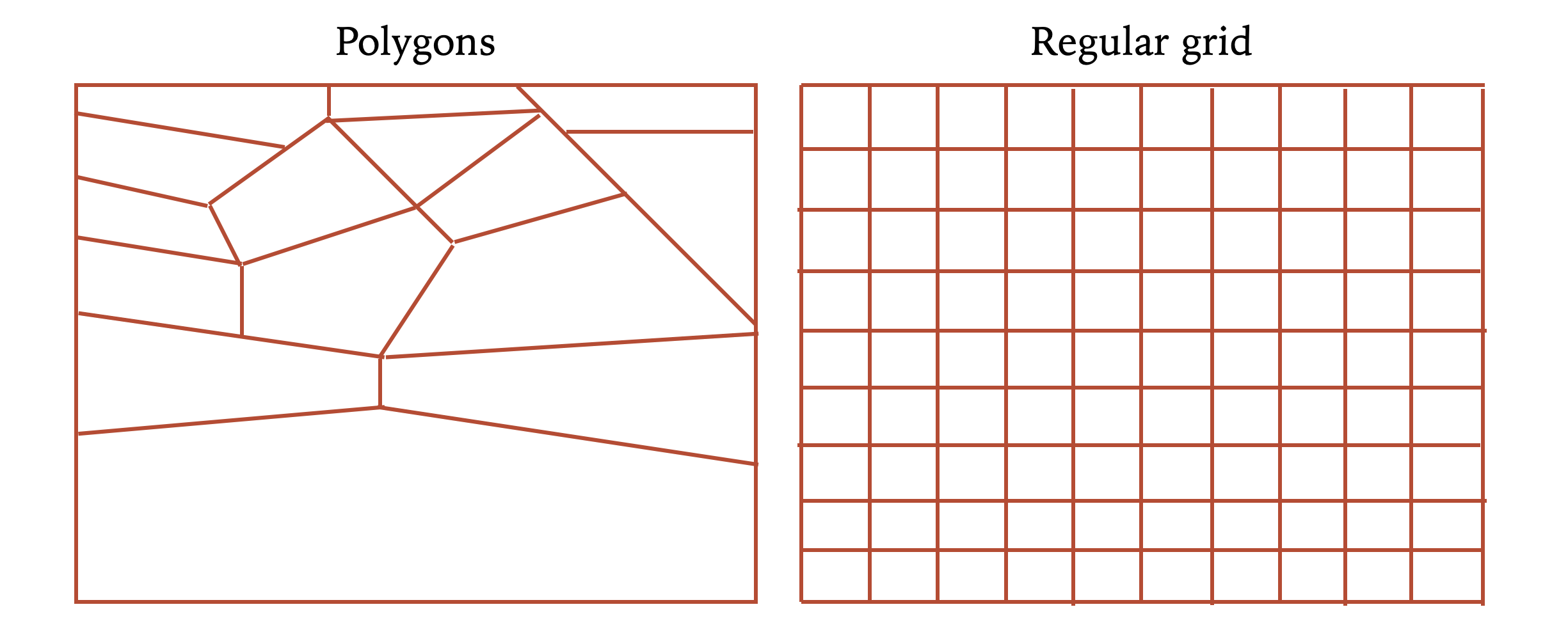
Figure 2. Polygon vs. regular grid domain spatial structure. Both types are used for ecosystem models, e.g., polygons for Atlantis and regular grids for Ecospace.

Using polygons make it simple to interpolate over larger area with generally much fewer cells required to describe the spatial characteristics of a model domain.  But it comes at the price of having to estimate how much flow there is between cells that only overlap partially (Figure 1).  On the upside, polygons calls for much fewer cells – take for instance a model of a country’s EEZ stretching 200 n.miles out from the coast. The core dynamics and fisheries will be in the perhaps narrow coastal zone with detailed habitat structures, while the offshore area will be much more uniform and with focus on the pelagic zone. Such a domain could with polygons be defined with more polygons in the coastal region and only few in the offshore. when using regular grid, the same resolution must be used throughout.

What to choose then? For the spatial model of EwE, we have chosen a regular grid based on an evaluation of the computational cost involved in keeping track of the exchange between irregular cells.  The “everybody loves pretty maps” argument was not instrumental in the decision, but the regular grid does offer some advantages when it comes to describing for instance the impact of placing alternative energy platforms in an ecosystem. It’s straightforward to evaluate alternative scenarios with the regular grid compared to a polygon system. Also, we’ve found that the regular grid makes it really straightforward to develop alternative model resolutions in one go. When constructing spatial layers, we often make them with different resolutions in one go, so that when running the models we start with a low resolution grid to start getting the models to behave, then shift to an intermediate when the model is more tamed, and finally to a high resolution for the production runs. Generally, the results don’t change between the medium and high resolution runs, but … everybody loves pretty maps!

Dimensionality

Time is the fourth dimension, but how many dimensions to you need for your ecosystem model?  That (as you’ll know already) depends on your policy/model question. The general answer is as few as possible, nothing new about that either.

If the question relates to water movements, we really have no choice but to go for a 3D model. It is necessary to capture how flow fields will the impacts are temperature patterns, a.o. We use hydrodynamic models for that.

But what about ecosystem models? 3D comes at a cost of one to two orders of magnitude in run time compared to a 2D model, so what’s preferable, 2D or 3D? There is no definitive or correct answer to that question, there are trade-offs. Plankton move up and down in the water column daily, and whales may dive to the bathypelagic zones in minutes. In consequence, we decided to go 2D for the spatial model of EwE, to stick to the map, not go 3D.  This is both for computational speed (see Run time below), but also because it isn’t really necessary to answer the type of policy/research questions we have seen posed to models.

Why not 1D to make it even simpler? One-dimensional models in the form of transects do indeed have a role to play, and in a 2D world they can easily be constructed. It’s more complicated to change a 1D model to 2D, so that’s another reason for the spatial EwE model being 2D.

Time step

The 3D vs 2D debate also has consequences for what time step to use.  The general rule is that particles or organisms should only be able to move to the nearest neighbour cell within a time step, not across multiple.  For 3D models that often have a large number of layers in the vertical zone this typically means that the time step is measured in minutes. That is a problem for ecosystem models where they dynamics of key species of interest may well be captured with time step measured in months.

For the spatial EwE model, the default time step is indeed a month, so 12 time steps per year, which is the time unit used for rates such as the production/biomass ratio.  For the vast majority of the questions asked of ecosystem models with focus on human impacts, such time lines are indeed what is called for.

May be added, that if the policy/research question calls for for instance analyzing short term aspects, this can be accommodated straightforwardly by simple changing the unit of the Ecopath input rates from annual to a finer scale. E.g., using daily rates will result in Ecospace time steps of 24/12 = 2 hours.

It should be noted that Ecospace is not appropriate for explicitly modeling the very fine scale horizontal and vertical movement/mixing processes (10’s of meters, hours to days) that create foraging arena vulnerability exchange relationships.  The effects of such relationships are already represented in the Ecosim model search rate and vulnerability exchange parameters, including such effects as limited diurnal overlap by vertically migrating foragers and/or their prey.  A few people have tried to use Ecospace to explicitly model movement for example between spatial patches representing predation refuges and other patches where foraging takes place.  This creates both a double-accounting problem for trophic interaction rate predictions and also typically a really fine spatial grid with huge computational requirements per time step.

Run time

While last in this chapter, it is not least. It matters how long time it takes to run a spatial model. Spatial ecosystem models are complex beasts (in contrast to physical models where behaviour isn’t a factor), and we will never^[5] be able to tame such models without trial and error, i.e. without exploring the input parameter space and evaluation model performance.  In practice this calls for model run time to be short enough to make multiple runs with output exploration feasible.

Quiz