Tutorial: Ecospace maps

So, you have an Ecospace model, it looks good, well, on the screen it does, but how do you make publication ready plots? That’s what this tutorial intends to give you some hints about.

In the process we’ll be using some GIS maps for the study area, but unfortunately we only have low-resolution maps of Anchovy Bay (and no GIS map for overlay), so we’ll use a colder study area, the Barents Sea. There, snow crabs have been expanding, and we’ll produce some maps to visualize how their distribution has changed.

We have a spatial model for the area, developed as part of the EISA project, coordinated by NIVA. Open your Ecospace scenario, the go Menu > Tools > Options > File management, and check the Ecospace > Run results > Biomass maps (ASCII format) option. Make a run, and Ecospace will save ASCIII raster maps to the directory that is specified on the File management form. That’s a lot of files being saved, by the way, so we need some reasonably smart way of handling them.

Let’s attack this using R. Get R up and running, make a folder for your mapping code, create an empty R file and save it. Copy the ASCII files you want to work with to a subfolder, in this example named asc.

# Then load libraries (install as needed):

library(terra)        # for spatial operations

library(viridisLite)  # colour blind friendly scheme for plotting

library(viridis)      # colour blind friendly scheme for plotting

# Next set your working directory:

#============= Set up working directory =============================

work.dir = dirname(rstudioapi::getActiveDocumentContext()$path)

setwd(work.dir)

# We need some colours to work with, here they are in a block:

# =======We need some colours to work with ========================

colrD=viridis(n=128,begin=0, end=1, direction=-1, option=”C”)

for(ix in 1:3) {colrD[ix] = “#FFFFFF”}

# =======end of colours ===========================================

# Let’s tell R where to find the ASCII maps:

files.start = list.files(path=”asc”

                         ,full.names=T,pattern=glob2rx(“EcospaceMapBiomass-some-crab*.asc”) )

# And let’s count how may files there are in the folder:

how.many = length(files.start)

# We’ll need a background to mark the area outside of our study area

backgr = rast(files.start[1])

values(backgr) = 0  #cells outside study value needs to get a value (will be NA otherwise)

# Find the max biomass on any map for scaling maps:

maxv=0

for(i in (1:how.many)){

  bef = rast(files.start[i])

  max.bef = max(setMinMax(bef))

  maxv = max(max.bef,maxv)

}

# Get a map of land to put on top of Ecospace map, this makes it much easier to see where your area is (compare Figure 1 B and 1C, below):

land = rast(“land_10k.asc”)

# Let R know your file name and type

pdf(file=”Four strong maps.pdf”,width=6,height=8,bg=”transparent”)

# We here want four plots for demo:

par(mfrow=c(2,2))

# Set margins to make plots fill the space better

par(mar=c(0,0,0,0))

par(oma=c(0,0,0,0))

par(xaxt=”n”, yaxt = “n”, bty=”n”)

# There are so many files, we only want to select some:

for(i in seq(11,how.many,by=6)){

  plt = rast(files.start[i])

  # first plot a grey background (Figure 1 A)

  image(backgr,xlab=””,ylab=””,useRaster=T,cex.main=2,zlim=c(0,1),col=”grey70″)

  # use the same scale for all plots (Figure 1 B)

  image(plt/maxv,xlab=””,ylab=””,add=TRUE,useRaster=T,cex.main=2,zlim=c(0,1),col=colrD)

  # add land on top of plot (Figure 1 C)

  image(land,xlab=””,ylab=””,add=TRUE,useRaster=T,cex.main=2,zlim=c(0.5,1),col=”grey30″

  # check the plot to find the X-Y coordinates for where to place a legend on top (Figure 1 D)

  year=as.character(1984+i)

  text(700000,-2300000,year,col=”white”,cex=2.5)

}

# turn off the device to save the pdf

dev.off()

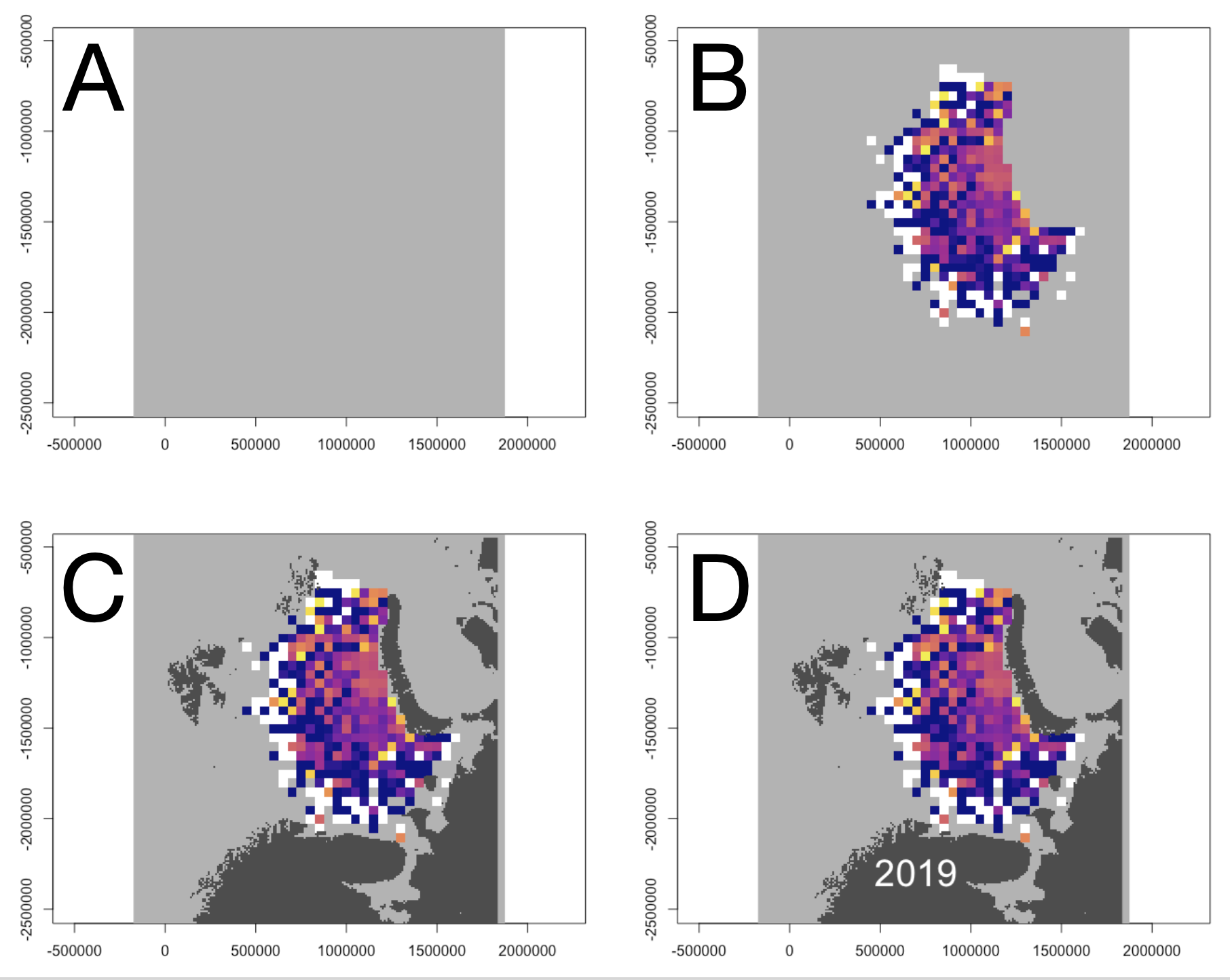
Figure 1. Maps of species distribution showing four stages of the plotting as described in text above.

That’s it, you now have some sample code with which you can read Ecospace maps and plot it.

What about Anchovy Bay?

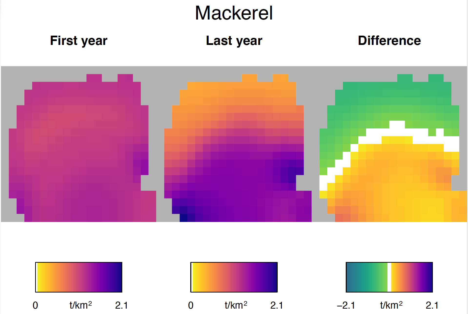
Figure 2. Map of mackerel biomass in Anchovy Bay at the first and last year of the model run, along with the difference (last-first) in the third plot.

Anchovy Bay should not be left out, so we’ve stored the R-code for the plots at the link in the textbook below. You should be able to download the code, place it in a folder, then open the R-code, run the model, and it should produce the plot. The plots will be in the pdf sub folder.

To use the code for your own plot, you will need to

• Run your model in Ecospace set to save: Click the floppy disk icon, then check Ecospace > Run results > Biomass maps (and any other maps you may want to plot)
• Line 20, set filedir = the folder where you have stored your Ecospace ascii files (.asc)
• Line 23, check the ascii files and get the first map about one year into the run (probably named 013). Set mth1 = “013” (or whatever yours is called, enter as string, i.e. with “” around the number)
• Line 25, set mth2 = the last month in your data files (e.g., “481”)
• Line 27, enter title for the first set of plots
• Line 29 Enter title for second set of plots

That’s all, the code should produce a pdf for each group in your model.