Tutorial: Incorporating environmental forcing
Learning Objectives
-
Obtain experience with how to incorporate environmental preference functions in EwE
We will, once again, use the ecosystem model of Anchovy Bay that we constructed in a previous tutorial (download). The purpose of this exercise is to incorporate environmental effects using environmental preference functions.
In preparation for this tutorial, please read the section about incorporating environmental forcing as well as the paper describing the underlying habitat capacity model[1].
Modelling impact of changing environmental conditions
Ecosim and Ecospace both have a flexible way to incorporate environmental effects. One can define an environmental preference function and in essence let the productivity (or other factors) be impacted by for instance temperature, O2, or pH. To illustrate the capabilities, we:
- Set up Ecosim to use the forcing function T bottom (bottom temperature) that is included in the Anchovy Bay time series file in Table 1 (below, or download) to force temperature over time.
- Set up Ecosim to use an environmental preference function that will translate the impact of changing temperature for one group in the system (here: whiting)
Environmental forcing function
When using environmental preference functions (such as temperature, O2, salinity) they should be read in with the appropriate units, so, e.g., temperature in ˚C – not relative to the baseline temperature. For this exercise we will use bottom temperature, which can be read in as annual values and included in a time series file (see Table 1).
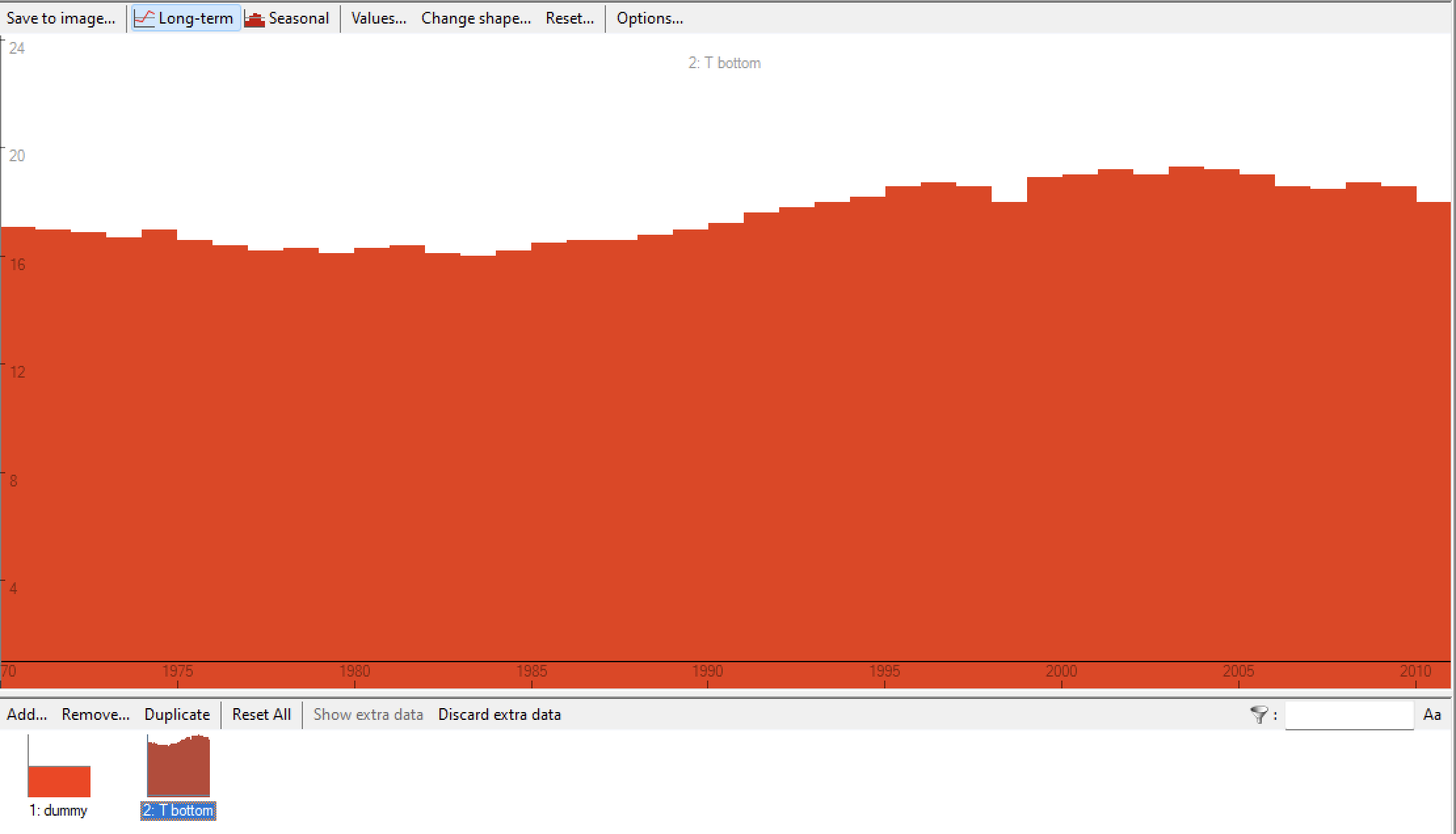
Check your model (Ecosim > Input > Forcing function) and load a time series (the one called anchovybay T in the downloaded database) to make sure you have the “T bottom” temperature read in. If not, read it in from the CSV file (below, or download).
 Figure 1. Screenshot (Ecosim > Input > Forcing function form) of forcing function “T bottom” read in via a CSV time series file. The function has annual bottom temperature values for Anchovy Bay. If preferable, monthly temperatures could be read in instead.
Environmental preference function
We next set up the preference function. Click Ecosim > Input > Environmental responses. Next click Add (in the lower left section of the form at the right) to add a new functional response function, double click on the name of the new function (at the bottom of the lower left panel), and a form Change shape should pop up. Change the shape name to, e.g., “whiting T” as we now will setup a temperature preference function for whiting to illustrate the approach. Then select Trapezoid, and set left bottom to 10, left top to 15, right top to 16 and right bottom to 19. Note that any shape can be defined (preferably based on data); the present example is for illustration only. Press OK.
Figure 2. Ecosim > Input > Environmental responses > Change shape form.
Next click Define response, and,
- If not done already, set X min to 10 and X max to 19.
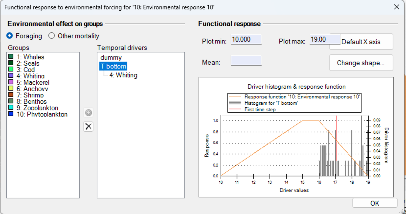
- Click Whiting in the Group panel and click T bottom in the Temporal drivers’ panel, then click the arrow between the two panels to assign whiting to the bottom temperature function. You should now see a histogram with the temperature distribution from the forcing function – the histogram is for information and can help ensure that your function is in the right range
- Set X min to 10 and X max to 19 (˚C; units not shown). Click OK to close the pop-up form.
 Figure 3. Ecosim > Input > Environmental responses > Define response form. If you cannot change the Plot min and Plot max: do it on the Ecosim > Input > Functional responses grid
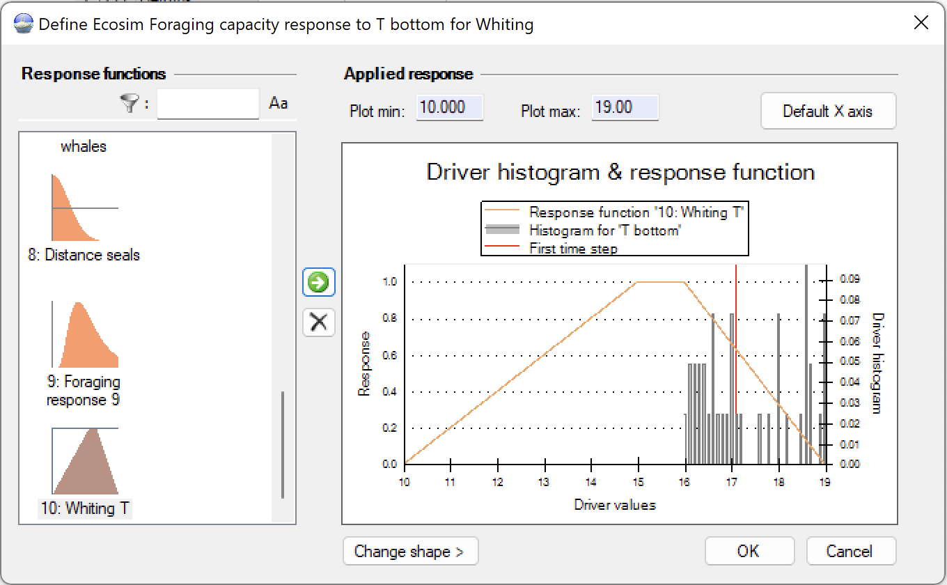
Next, click Apply environmental response (foraging), and check that T bottom has been applied to Whiting. If not, click the cell that intersects T bottom and whiting. On the pop-up Define Ecosim foraging capacity response form, find your “Whiting T” shape, click the green arrow to move it to the right side (and apply it), see Figure 4.
 Figure 4. Application of Ecosim foraging response.
Now run the model with and without the forcing function (you can disable it on the Figure 4 form by selecting the x between the two panels, run, extract results; apply again, run, extract results), and evaluate the impact of using this forcing function and environmental preference function.
On Ecosim > Output > Run Ecosim, click the Save output button (floppy disk) below the top menu, and check Ecosim > Run results. Run Ecosim (time series fitted version) and extract the biomass trends by group (click the save button floppy disk discussed above, and click the little yellow folder to the right of the Run results. This should open Windows Explorer with the folder where the biomass results are stored). Open the file biomass_annual.csv. Save the csv file to a different directory (to avoid overwriting it).
The Anchovy Bay model has a number of environmental preference functions, see Ecosim > Input > Environmental responses, including ones called Temp cold and Temp warm. In the Ecosim > Input > Environmental responses > Apply environmental response foraging, select the cell that intersects Cod and bottom T, and transfer the Temp cold function to the Applied responses. Do similar for the intersect between Anchovy and bottom T, and transfer the Temp warm function.
Run Ecosim and extract the biomass trends by group. Save the output files (as above). Compare the biomass trajectories by species with and without the environmental preference functions applied.
Table 1. Time series file for the Anchovy Bay tutorial. You may already have this CSV file from the Time Series Fitting tutorial, if not, you can download it here, or copy the content below, paste it into MS Excel, then save it as a CSV file. Import the CSV file to EwE as described in the tutorial.
| Title | Sealers | Seal B | Trawlers | Cod B | Whiting B | Shrimp C | T bottom | dummy |
| Weight | 0 | 1 | 0 | 1 | 1 | 1 | 1 | 1 |
| Pool code | 1 | 2 | 2 | 3 | 4 | 7 | 5 | 4 |
| Type | 3 | 0 | 3 | 0 | 0 | 6 | 2 | 2 |
| 1970 | 1 | 1 | 1 | 10 | 1 | 0.3 | 17.1 | 1 |
| 1971 | 1 | 1.05 | 17 | 1 | ||||
| 1972 | 1 | 1.103 | 16.9 | 1 | ||||
| 1973 | 0.75 | 1.158 | 16.7 | 1 | ||||
| 1974 | 0.5 | 1.216 | 17 | 1 | ||||
| 1975 | 0.25 | 0.8 | 1.276 | 16.6 | 1 | |||
| 1976 | 0 | 1.34 | 16.4 | 1 | ||||
| 1977 | 0 | 1.407 | 16.2 | 1 | ||||
| 1978 | 0 | 1.477 | 6 | 0.8 | 16.3 | 1 | ||
| 1979 | 0 | 1.551 | 16.1 | 1 | ||||
| 1980 | 0 | 1 | 1.629 | 16.3 | 1 | |||
| 1981 | 0 | 1.71 | 16.4 | 1 | ||||
| 1982 | 0 | 1.796 | 16.1 | 1 | ||||
| 1983 | 0 | 1.886 | 16 | 1 | ||||
| 1984 | 0 | 1.98 | 16.2 | 1 | ||||
| 1985 | 0 | 2.079 | 16.5 | 1 | ||||
| 1986 | 0 | 2.183 | 16.6 | 1 | ||||
| 1987 | 0 | 2.292 | 16.6 | 1 | ||||
| 1988 | 0 | 2.407 | 16.8 | 1 | ||||
| 1989 | 0 | 2.527 | 4 | 0.7 | 17 | 1 | ||
| 1990 | 0 | 2.577 | 17.2 | 1 | ||||
| 1991 | 0 | 2.629 | 17.6 | 1 | ||||
| 1992 | 0 | 2 | 2.682 | 17.8 | 1 | |||
| 1993 | 0 | 2.735 | 18 | 1 | ||||
| 1994 | 0 | 2.79 | 18.2 | 1 | ||||
| 1995 | 0 | 2.846 | 18.6 | 1 | ||||
| 1996 | 0 | 2.903 | 18.7 | 1 | ||||
| 1997 | 0 | 2.961 | 2 | 0.6 | 18.6 | 1 | ||
| 1998 | 0 | 3.02 | 18 | 1 | ||||
| 1999 | 0 | 3.08 | 18.9 | 1 | ||||
| 2000 | 0 | 3.142 | 19 | 1 | ||||
| 2001 | 0 | 3.205 | 19.2 | 1 | ||||
| 2002 | 0 | 3 | 3.269 | 19 | 1 | |||
| 2003 | 0 | 3.334 | 19.3 | 1 | ||||
| 2004 | 0 | 3.401 | 19.2 | 1 | ||||
| 2005 | 0 | 3.469 | 1 | 0.4 | 2 | 19 | 1 | |
| 2006 | 0 | 3.5 | 18.6 | 1 | ||||
| 2007 | 0 | 3.5 | 18.5 | 1 | ||||
| 2008 | 0 | 3.55 | 18.7 | 1 | ||||
| 2009 | 0 | 3.6 | 18.6 | 1 | ||||
| 2010 | 0 | 4 | 3.65 | 2.4 | 18 | 1 |
Media Attributions
- Ecosim > Input > Forcing function
- Ecosim > Input > Environmental responses > Change shape
- Ecosim > Environmental responses > Define response form
- Ecosim > Input > Environmental responses > Apply environmental response (foraging)
- Christensen, V, M Coll, J Steenbeek, J Buszowski, D Chagaris, and CJ Walters. 2014. Representing variable habitat quality in a spatial food web model. Ecosystems 17(8): 1397-1412 ↵

