Tutorial: Policy exploration procedure
Villy Christensen and Santiago de la Puente
About this tutorial: It is intended for more complex applications of the fishing policy module rather than for introductory EwE courses. There's a simpler tutorial to start with (link).
Preparation: Read the Fishing policy optimization chapter (see chapter) and the User Guide interface description (see chapter) before embarking on this tutorial.
The EwE policy exploration module is a complex but capable beast, designed for policy exploration of trade-offs, not for providing management advice for direct implementation. The policy advice it can produce is strategic rather than tactical (i.e. broad, directional policy advice rather than specific management advice). It can thus contribute at the table where policy discussions take place, in particular by providing options for and trade-offs in ecosystem-based management.
In this tutorial, we'll go through and explain details for how the module may be used for actual policy exploration. As part of this, we will outline, step by step, a procedure we find useful for conducting a more complete policy exploration that can be published and potentially can contribute to policy development.
Model scope and behaviour
We assume that your model is indeed to be used for actual policy exploration, and advise that the model, while being predictive (rather than descriptive, see the Defining the ecosystem chapter) should include the fleets among which the policy module will seek to balance trade-offs – this may well be all fleets operating in the given ecosystem as trade-offs often are through food web interactions and bycatch. Further, the target species for the fishery should be included in the model, along valued species that they take as bycatch, along with their prey and competitors, and where applicable top predators such as marine mammals and species of conservation concern.
For the model behaviour in response to proposed fisheries changes it is important that the model is fitted to time series data – this implies that density dependence related to carrying capacity has been considered (see Density dependence and carrying capacity chapter), and the vulnerability multipliers that affect population resilience have been modified accordingly, (see Vulnerability and vulnerability multiplier chapter).
It should hardly come as a surprise that we use Anchovy Bay for illustration in this tutorial. If needed, you can download a version of the Anchovy Bay model that is fitted to time series data from this link. This is the version that is used for this tutorial.
Note though that the time series fitting is rather incomplete in this version of the Anchovy Bay model, e.g., effort is lacking for several fleets.
Fleet considerations
If you have fleets in your system that it does not make sense to optimize for, e.g., optimizing for profit for a recreational fleet or a "catch-all" IUU[1] fleet, they can be considered in optimizations without being included in optimization searches. For this, on the Blocks form in the interface select the first (black) block, then click the name of the fleet in the spreadsheet, and all years will be blackened out. When this is done, the Ecosim effort will remain as entered for that group, but the calculations of objectives will still include impacts of and on the blocked fleet(s).
As an example, the recreational fleet may be relying on a species that is also a target for a commercial fleet that is considered in the optimizations. Abundance changes caused by changing the commercial fleet effort will then impact the catch rates of the recreational fleet, which in turn will impact optimization measures that are affected by the recreational fleet.
For evaluating the Social value (employment) objective, it is important to set the relative Jobs/catch value parameters in the Ecosim > Tools > Fishing policy search table. By default these are at unity (1) for all fleets, which is a reasonable assumption for Anchovy Bay (so we will leave all Jobs/catch value at 1 for this tutorial), and indeed perhaps for many other places. Still, this parameters is important and it is best if you can use local or regional data.
Time period: retrospective or forward?
There are two different approaches that have been used for policy optimizations, retrospective analysis vs. forward-looking scenarios, and we will describe both in the present extended tutorial.
The general advice is, where possible use forward-looking scenarios, but if for some reason this isn't feasible, the retrospective analysis is also a good option.
Retrospective analysis
For this, the idea is to explore a what-if of the kind "how might the situation in this system have developed if the policy objectives had been implemented throughout the historic time period". This allows fitting of the model to time series data and to include environmental productivity patters. So, here we know what happened and we compare that to what might have happened if we had optimized the fisheries from early on.
Forward-looking scenarios
For these, the idea is to use a model that has been fitted to time series data, running up to the present. We then explore what options we have looking forward to explore alternative policy optimization scenarios. We may for instance add 20 years[2] to the runtime in Ecosim (Ecosim > Input > Ecosim parameters > Duration of simulation), then on the Ecosim > Tools > Fishing policy, click the black colour in the Blocks section, and block the historic time period for all fleets so that the optimizations will only be done for future years.
Forward-looking scenarios beg the question of how to handle a changing environment. The often-taken approaches for this are,
- Make the policy optimizations on the background of no change, i.e. keep the environmental productivity and patterns as they were at the end of the historic period,
- If you have environmental productivity patterns, then repeat those pattens going forward,
- Use output from climate models to drive the Ecosim environment.[3]
Exploratory analysis
Objective ranges
Policy explorations are often intended to explore less extreme, more balanced solutions for fleet tradeoffs. That calls for using weights on several policy objectives (see textbook Policy exploration chapter) – but what weights are needed to make the resulting fishing efforts "balanced"? Using the same weight (e.g., 1) for all objectives is not likely to results in a reasonable balance of performance measures. What then?
When you are ready to explore the policy optimization, the first step is to evaluate the range of optimized fishing efforts that result for each objective. Open your model (or Anchovy Bay from this link), load the Ecosim scenario you want to use, but do not load time series. Then run four policy searches with default settings varying only the objective weights. In the first search give the Net economic value a relative weight of 1, and leave the relative weight on all other objectives at 0. In the second run, give the Social value (employment) a value of 1, and all others 0. Then third and fourth runs are with only weights on Ecosystem structure and Biodiversity, respectively.
There is no need to include the Mandated rebuilding objective in the range of tested optimizations as this objective differs in behaviour, and serves a purpose different from other objectives. When invoked it is either, (1) a forced rebuilding or (2) providing a limit for the minimum acceptable biomass (Blim/B0)[4]. This objective is thus intended to take precedence over all other objectives, and it should have a weight that trump all other objectives, (so very high, e.g., 100). The Mandated rebuilding is functional group specific, and only impacts the optimization when the biomass of a specified group falls below a user-defined reference level (Blim/B0). When the biomass is at or above Blim/B0, the objective has no impact on the optimization.
For Anchovy Bay, we may get results as in Table 1 from the single objectives optimization runs.
Table 1. Policy optimization objective ranges for four runs, each with weight on only one objective at the time.
| Optimizing for \ Objective | Econ. | Social | Ecosys. | Biodiversity |
|---|---|---|---|---|
| Econ. | 1.84 | 1.15 | 0.96 | 1.02 |
| Social | (2.26) | 2.34 | 0.59 | 0.88 |
| Ecosys. | 1.28 | 0.68 | 1.32 | 1.05 |
| Biodiversity | 0.71 | 0.50 | 1.08 | 1.05 |
| Min. value | - | 0.50 | 0.59 | 0.88 |
| Max. value | 1.84 | 2.34 | 1.32 | 1.05 |
| Range | 1.84 | 1.83 | 0.73 | 0.17 |
| 1 / range | 0.5 | 0.5 | 1.4 | 5.9 |
Table 1 shows the outcome from the four objective-by-objective runs. The range of objective values are indicated (ignoring negative Net economic values) and make it clear that the two economic objectives have the largest range, followed by Ecosystem structure. The Biodiversity objective has a much more narrow range. There is no truth or absolute values coming out of this exploratory analysis, but it serves to illustrate that using equal weight on all objectives is unlikely to lead to a balanced solution. Instead, as a first estimate for weights to use across fleets one may be able to use the inverse of the ranges, see Table 1.
Using the inverse of the objective range may lead to a more “balanced” outcome during optimization exercises as this scaling better reflects the how "easy" it is for each objective to influence the objective function. This should, however, not be taken to mean that using the inverse range represents the truth, the whole truth and nothing but the truth: it is merely a more reasonable starting point than assuming the using the same relative weight for all objectives is a balanced solution.
If a search is stuck with negative profit
It can happen when you start running optimizations with the "limit cost > earnings" option, that both the net economic value and the social indicator (jobs) are negative already at the two initial runs. This indicates that a penalty has been applied in the search routine where the penalty increases rapidly as the ratio cost/income increases toward and exceeds 1.0. Such a penalty is needed to make the optimization move away from fleet efforts that drive cost > earnings.
When it happens from the onset, it indicates that the baseline effort is unsustainable. In the case of Anchovy Bay, the culprit is the sealers fleet, which has a high, unsustainable effort in the base year. In Ecosim run, the fleet is shut down after a few years, but in the optimization, the high initial effort is maintained through the run. The optimization takes the cost and value at the baseline and sums the cost and value at the last year, and it multiplies that last year with a discounted value of what the last years catch would be worth if it were continued for an additional 20 years (i.e. there's a high weight on the end state relative to the baseline).
In some cases, the optimization routine can find its way out of the unsustainable fleet effort range, but not always. If the routine keeps producing negative indicators for the first two objectives, try making a run where you flatline the effort (1 throughout), and see which fleets end up having negative profit in the last year. Then reduce the effort for those fleets, and run the optimization again.
Searches with "limit cost > earnings" may have issues, and are not at all guaranteed to work. Consider if you can get by without using this option if there are problems with this in your model.
When running the policy optimization for Anchovy Bay with objective weights = the inverse of ranges from Table 1, the results in the table below are obtained.
Table 2. Objective function values and fleet effort for a retrospective optimization for Anchovy Bay with weights set to inverse range of objectives. Optimization started with Ecopath base effort.
| Total | Econ. | Social | Ecosys. | Biodiversity |
|---|---|---|---|---|
| 3.70 | 1.69 | 1.08 | 1.05 | 1.02 |
| Sealers | Trawlers | Seiners | Bait boats | Shrimpers |
| 0.89 | 1.66 | 0.72 | 0.85 | 0.59 |
Introducing priors for weighting schedules
This type of weighting schedule perhaps best illustrates the outcomes of broad policy goals such as “securing the triple bottom line” or “promoting profitable, sustainable and just fisheries”.
Granted that this discourse has become more mainstream, we are work under the assumption that fisheries stakeholders and the civil society are generally aiming for sustainable futures. However, different stakeholder groups will have different ways of weighting objectives, within and across fisheries systems. For example, fishers in some location may want to maximize fisheries rent twice as much as ecosystem structure, while recreational divers in another may want to maximize biodiversity 50% more than social benefits and 90% more than fisheries rent.
Published literature using EwE’s policy search routine has addressed this by building scenarios where different weighting schedules are applied to represent a “compromise” among stakeholder objectives.[5] However, grounding scenarios with field data is something that modellers should strive for. To adequately capture people’s viewpoints, researchers should collect primary data (e.g., through semi-structured interviews or surveys) that allows them to construct alternative weighting schedules for different types of stakeholders operating in the system. This requires questions that rank optimization objectives and map the relative distance between them.
For instance, let’s say that a survey was implemented along the multiple communities that inhabit Anchovy Bay. The goal was to gather data on the policy preferences of coastal dwellers rather than those of the more “usual suspects” of fisheries systems (e.g., fishers, seafood processors, distributors, or sellers). People were asked to agree with certain statements (e.g., “Economic growth must be a priority for the my country, even if it affects the environment” or “Fishing effort should be restricted to prevent overfishing, even at the expense of losses in employment"), and the answers were arranged using a 5 point Likert scale with options ranging from “Strongly disagree” to “Strongly agree”. As questions addressed all permutations among objectives included in the policy search routine, we created a distance matrix for them and used it to rank them.
Inhabitant of Anchovy Bay prioritized maximizing ecosystem structure as the central objective of local fisheries policies. This objective was closely followed by maximizing biodiversity, and more loosely followed by employment and revenue considerations. For the sake of simplicity, no questions addressed the mandated rebuilding objective. Inhabitants of Anchovy Bay are thus more pro-environment than the fishers, and certainly more in favour of conservation than local politicians believe their constituents to be. Using the responses we created an index where the objective with the highest value was given a value of 1, and all other objectives were scaled to it based on their relative importance, which leads to the weightings in Table 3. These values can then be used as multipliers for the weights of the objectives used in the “balanced” outcome run, to skew them towards their preferences and highlight the differences.
Table 3. Relative weighting as obtained from interviews with Anchovy Bay community members. The table also shows the inverse weighting from Table 1 and the resulting combined weight, which is the product of the community weighting and the inverse weighting.
| Objective | Rel. weight | Inverse weighting | Combined rel. weight |
|---|---|---|---|
| Economic rent | 0.56 | 0.5 | 0.3 |
| Social benefits | 0.75 | 0.5 | 0.4 |
| Ecosystem structure | 1 | 1.4 | 1.4 |
| Biodiversity | 0.94 | 5.9 | 5.5 |
Table 4. Objective function values and fleet effort for a retrospective optimization for Anchovy Bay with weights set to the combined weigthings from Table 3. Optimization started with Ecopath base effort.
| Total | Econ. | Social | Ecosys. | Biodiversity |
|---|---|---|---|---|
| 3.98 | 1.33 | 0.81 | 1.38 | 1.04 |
| Sealers | Trawlers | Seiners | Bait boats | Shrimpers |
| 0.05 | 1.21 | 0.03 | 0.46 | 0.62 |
Comparing Table 2 and Table 4, it's noticeable that adding the strong conversation-oriented view of the Anchovy Bay community has some socio-economic consequences. The economic rent and social benefits performance values were reduced with 20-25%, the ecosystem structure indicator increased ~30%, while the biodiversity measure (which is relative hard to impact) increased with a couple of percent.
If you want to explore the effect that the two optimizations have on fleet catches and values, and on group biomasses, you can extract that information (after each optimization) from the tables on the Ecosim > Output > Ecosim results form.
Local maxima
As part of the exploratory analysis, it is important to check whether the maximization search is impacted by the start point, i.e. whether the optimization solutions are unique. By default the optimization routine will start with the fishing rates defined by the Ecopath baseline. It's possible, however, to instead using random fleet effort (Random F's in the policy interface) to check if the optimization routine is likely to get stuck at local maxima. All optimization routines are impacted by this, the ones in EwE being no exceptions.
We illustrate this for Anchovy Bay by running 70 optimizations with the combined rel. weights from Table 3, and runs initialized with random F's. The outcome of that exploratory analysis is presented in Figure 1.
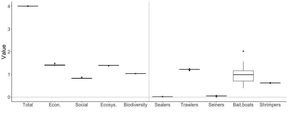
Figure 1. Box plot[6] showing minimum, first quartile, median, third quartile and max value of objective function value for indicators and relative effort for fleets for 70 policy optimizations run with random Starting F initialization. It's clear that only the relative effort for the bait boats varies between runs (with one run way higher than the 69 others), and that the optimizations overall are robust to local maxima.
From Figure 1, it is clear that for this version[7] of the Anchovy Bay model, there is very little tendency for the optimization to get stuck on local maxima. The variation in the objective estimates and effort patterns are very similar across all runs (apart perhaps from bait boat effort), with only a few runs indicating presence of local maxima.
That this Anchovy Bay model isn't prone to get stuck on local maxima should not invite complacency, but be seen as a warning that there may be local maxima. We ran the optimizations 70 times for Figure 1 to illustrate this point – but also to show that it rarely happens. Bottom line is, run your optimization a number of times (maybe 10 to 20), check how consistent the output is. Then run the model once, check if the outcome corresponds to the majority of the random runs. If it does, you're good to go.
The overall conclusion is that policy optimizations for Anchovy Bay are not very prone to get stuck on local maxima. This is also what we have found for many other ecosystem model optimizations, giving some comfort that the starting point isn't very critical. Still, this needs to be checked for all models, so including a search with random Starting F's should be included in all more serious policy explorations.
Fleet trade-off analysis
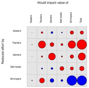
Figure 2. Fleet trade-off analysis for Anchovy Bay showing impact a 10% reduction in effort for the fleet listed in rows has on the fleets listed above columns. Negative impacts are in red, and positive in blue.
A next step of exploratory analysis is the fleet trade-off analysis described in the Fishing policy chapter (link to fleet trade-off). We refer to that section for description, including for code to produce plots.
We suggest that you perform the fleet trade-off analysis for your model and explore the outcome. For Anchovy Bay (Figure 2), the plot shows the impact that a 10% reduction for the fleets mentioned to the left, are predicted to have in the value of the catch for all fleets. Red circles indicate reduction in value, and blue increase. The impacts are displayed so that the circle areas are proportional to the changes in value of the catch, and are thus comparable across fleets[8].
For Anchovy Bay, the fleet trade-off analysis shows some both straightforward and more complex patterns. Notice for instance that a reduction in bait boats' effort will have a positive impact on seiners. That makes sense since the two fleets both catch anchovy. But conversely, a reduction in seiners' effort lead to a small reduction in landed value for the bait boats. Why? Seiners also catch mackerel, and the reduced effort will lead to more mackerel, which in turn will have a negative impact on anchovy, and hence on bait boats, (which only catch anchovy).
The strongest impact of effort reduction is for trawlers and shrimpers, the two fleets that have the highest value in the model base year. Reduction in trawlers' effort has a considerable negative impact on trawlers, but also an almost corresponding negative impact on shrimpers. That makes sense as the reduction should lead to more cod and whiting, both of which eat shrimp. But conversely, reducing shrimpers' effort leads to an increase in shrimp landings (so they must be overexploited in the baseline – given the baseline predator-prey conditions though). But why does this not lead to an increase in the value of trawlers' landings? The reason is that shrimp have a positive impact on whiting and mackerel, but a negative impact on cod. Notably, the increase in whiting impacts cod negatively. Those relationships becomes clearer if you check out the Mixed Trophic Impact analysis (Ecopath > Output > Tools > Network Analysis > Mixed trophic impact > Impact data), which shows that shrimpers have opposite impact on cod versus whiting and mackerel.
Your policy questions?
Having explored the behaviour of your model, e.g., as described above, the next issue is to clearly define what questions you are asking for your model. An example of this is Alms et al. 2022, [9] who compared output from three defined Ecosim scenarios, (1) ban on shrimp trawling, (2) gill net effort reduction of 25%, and (3) the combination of (1) and (2), and then compared these to the output of single- and multi-objective policy optimizations. Here, the multi-objective optimizations were designed to serve as more balanced solutions. See the paper for details.
Anchovy Bay
While the complex patterns in the fleet tradeoff (Figure 2) can be explained as above, they raise some questions. There is a big negative impact of reducing trawlers' effort and a big positive impact of reducing shrimpers' effort. Is this then what we should explore? Well, it's certainly interesting scenarios, but there are some complications, and it is in line with what actually happened in Anchovy Bay. Effort of trawlers indeed increased 2-3 times over time, but the shrimp effort increased by almost an order of magnitude. Does this make sense when the fleet trade-off analysis indicate that shrimp catches would increase if shrimpers' effort was reduced? The finding is not really wrong, but it doesn't not consider that the increase in the trawlers' effort reduced the abundance of cod and whiting, which in turn lead to many more shrimps being available for the shrimpers. Predator-release!
What the above indicates is in essence that the Anchovy Bay ecosystem of today is very different from that of 1970. Therefore, we will next run the policy optimization for Anchovy Bay as a forward-looking scenario where we keep the run from 1970-2010 as it was in the fitting, and then conduct the policy optimization from 2011 (year 42) onwards. Figure 3 illustrates the setup.
If you change the Ecosim > Tools > Fishing policy search > Base year to the end of the time series, the routine will automatically black out the years of the time series. In that case, the economic data (cost and value) in Ecopath > Input > Fishery > Fleets are assumed to represent your base year, not the Ecopath model year (Year 1 or 1970 for Anchovy Bay).
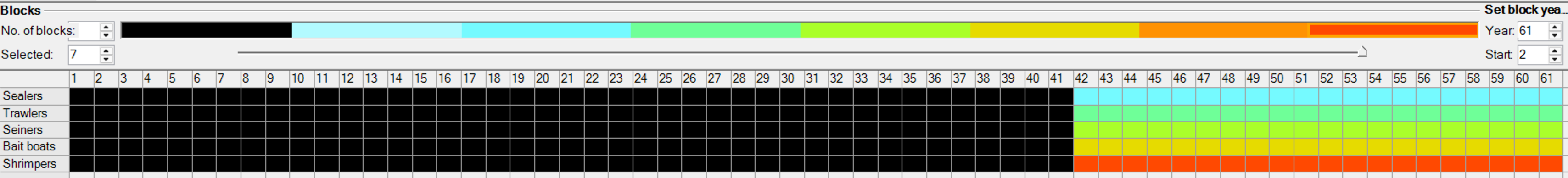
Figure 3. Fishing policy search interface set up to do a forward scenario for Anchovy Bay. The optimization will not change the effort for the first 41 years (in black), but search for one effort for each fleet for the last 20 years. If you cannot see all the years, try the zoom icons in the interface and widen the aspect ratio of the interface.
We run the forward-looking scenarios with Random F drawn to start the optimizations, which will ensure that we do not get stuck in a local maxima for all runs (even though we have found above that the risk of this is small). We here do not use the "limit cost > earnings" as this tends to hang the optimizations for the Anchovy Bay model[10].

Figure 4. Indicator values from Anchovy Bay model policy optimizations with inverse range weighting vs. community-based weightings (from Table 3). The community places higher weights on ecosystem structure and biodiversity, and the optimizations indeed reflect this. It's clear that all of the objectives contributes to the total objective function score, which is the sum of the four objectives – actually with less variation for the community-based weighting. But the improved ecological score is offset by lower employment and profit[11].
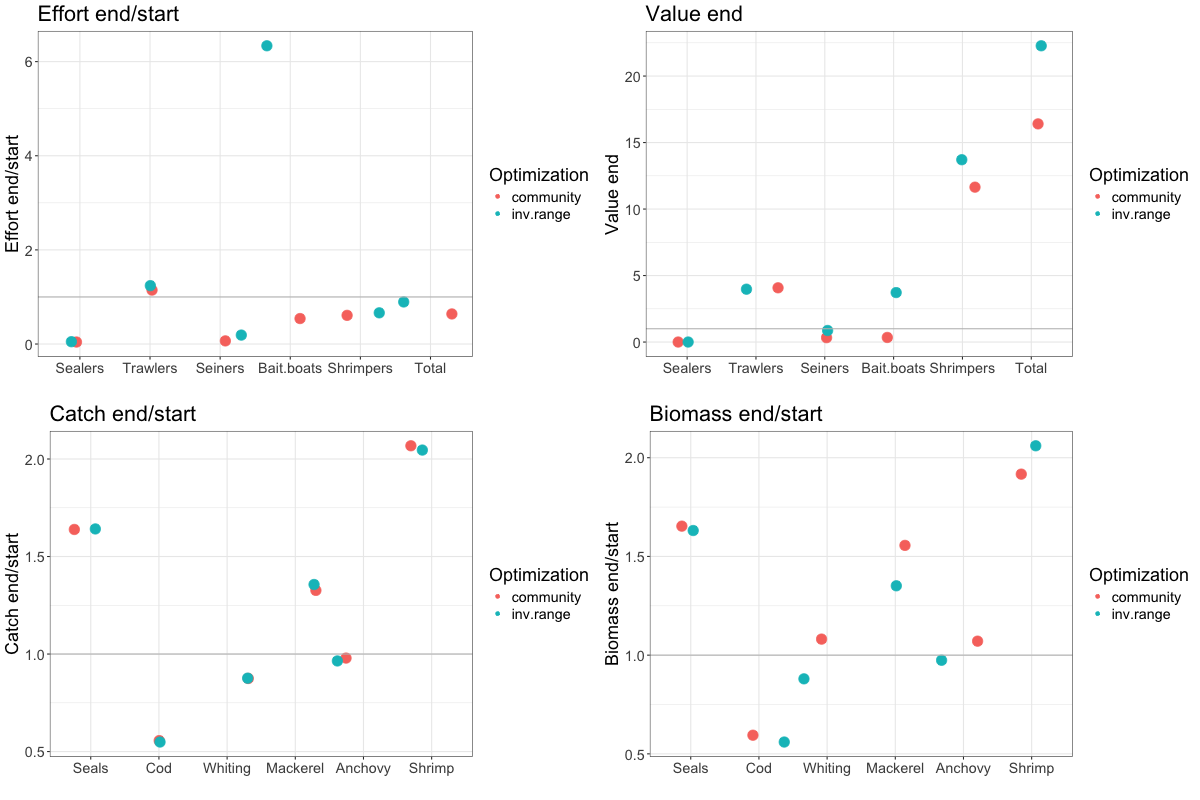
Figure 5. Plot[12] comparing fishing policy optimizations for Anchovy Bay model with weight as defined based on inverse range and community input in Table 3. Value is proportional to jobs, so the Jobs end plot indicates around a 25% reduction in jobs with the community-based weighting.
The fleet effort value, catch and biomass results for the Anchovy Bay model forward-looking policy scenario are presented in Figure 5, again comparing optimizations with the inverse range weightings vs the community opinion based weightings (both from Table 3). The results show the complex trade-off patterns between the two weighting schemes.
Your case
We suggest that you as a starting point go through this extended tutorial and conduct policy optimizations on a fitted version of your ecosystem model, working your way through the steps described in the tutorial.
Pretty good yield
When you run optimizations, you'll often see that the objective function may rather quickly get to more than 98% of the final objective function score. If you start with Ecopath base F, the effort changes may be rather limited when you pass the 98% mark, but the last few percent may cause big changes in effort. It may be worth exploring those intermediate states (by stopping the optimizations before it finishes by itself).
This is to some degree related to the idea behind Ray Hilborn's Pretty Good Yield[13] for MSY.
Acknowledgement
Media Attributions
- Original
- Original
- Ecosim > Tools > Policy search
- Original
- Original
- EcoScope logo
- Illegal, unregulated and unreported ↵
- Note that the policy optimization always runs for an additional 20 years without showing the results. This is to ensure that the optimizations do not result in an "empty sea" where fleets are encouraged to fish out the resources (which might happen if there was no tomorrow to consider). ↵
- This approach is used commonly for climate change scenarios, but may never have been used for policy optimizations. ↵
- Blim is the lowest acceptable biomass and B0 the Ecopath biomass for the group. The objective is thus entered as a relative biomass term. ↵
- e.g., Natugonza et al. (2020) https://doi.org/10.1016/j.fishres.2020.105593, and Alms et al., (2022) https://doi.org/10.1016/j.ocecoaman.2022.106349 ↵
- The R-code and CSV-file used for this figure can be downloaded from this link. ↵
- Optimizations depend on fitting and model parameters. Different versions of the Anchovy Bay may well lead to different optimizations ↵
- The monetary value of the fleet-tradeoffs can be obtained from the CSV file used for producing the fleet trade-off plots ↵
- Alms V, Romagnoni G, Wolff M. Exploration of fisheries management policies in the Gulf of Nicoya (Costa Rica) using ecosystem modelling. Ocean and Coastal Management 230 (2022) 106349. https://doi.org/10.1016/j.ocecoaman.2022.106349 ↵
- This is likely because we for this tutorial are using very rough economic data. If you have this issue, do check your assumptions about cost vs value in your base year. ↵
- R-code and data files to produce this code are included in the Zip file that can be downloaded for Figure 5, see below. ↵
- Download R-code and CSV-files used for Figure 4 and 5 from this link. ↵
- https://doi.org/10.1016/j.marpol.2009.04.013 ↵
